Does Volatility Scale With the Square Root of Time? Variance Ratio Test in Python

August 2, 2026

What’s the question?

Almost every risk number in finance rests on one shortcut. Take the standard deviation of daily returns, multiply by the square root of 252, and report the result as annualised volatility; multiply by the square root of 10 instead and a regulator accepts the answer as a ten-day value-at-risk input. Black-Scholes rests on the same assumption.

The shortcut is exact only when returns are serially independent. Variance adds across independent periods, so two days of variance is twice one day of variance and volatility grows with the square root of the horizon. Autocorrelation breaks that addition: when part of a move is given back the following day, multi-day variance grows more slowly than time.

The variance ratio test of Lo and MacKinlay (1988) measures the departure directly. VR(q) is the variance of a q-day return divided by q times the variance of a one-day return, and the square-root rule sets it to 1 at every q. Two things matter: how far from 1 real assets sit, and whether the gap survives sampling noise.

The approach

Six exchange-traded funds cover US large cap (SPY), US small cap (IWM), developed markets outside the US (EFA), long Treasuries (TLT), energy (XLE), and utilities (XLU), from January 2006 to December 2025: 5,031 daily total returns each.

1. Pull daily total returns and convert to log returns, so a q-day return is the sum of q daily numbers. Rows with a non-positive price or a daily return beyond plus or minus 50 percent drop first; none of the six triggered that bound.
2. Compute VR(q) at 2, 5, 10, 20, and 60 trading days with the overlapping estimator, which counts every start date rather than every twentieth and makes twenty years usable at a sixty-day horizon.
3. Compute the heteroskedasticity-robust z statistic, since volatility clusters in all six series and a standard error built on constant variance rejects the random walk far too often.
4. Repeat the one-month comparison using 251 non-overlapping 20-day blocks, a cruder estimator sharing no machinery with the overlapping one.

On 300 simulated random walks the estimator returned a mean VR of 1.00, so a ratio below 1 is not an artefact of the formula.

Code

import numpy as np
import xfinlink as xfl
from scipy import stats

xfl.set_api_key("YOUR_API_KEY")  # free at https://xfinlink.com/signup

ASSETS = ["SPY", "IWM", "EFA", "TLT", "XLE", "XLU"]
px = xfl.prices(ASSETS, start="2006-01-01", end="2025-12-31",
                fields=["adj_close", "return_daily"])
px = px.dropna(subset=["return_daily"])


def variance_ratio(x, q):
    """Lo-MacKinlay overlapping variance ratio with heteroskedasticity-robust z."""
    n = len(x)
    mu = x.mean()
    e = x - mu
    var_1 = (e ** 2).sum() / (n - 1)
    cum = np.concatenate([[0.0], np.cumsum(x)])
    qsum = cum[q:] - cum[:-q]                       # overlapping q-day sums
    m = q * (n - q + 1) * (1 - q / n)
    vr = (((qsum - q * mu) ** 2).sum() / m) / var_1
    denom = ((e ** 2).sum()) ** 2
    theta = sum((((2 * (q - j)) / q) ** 2) * n * ((e[j:] ** 2) * (e[:-j] ** 2)).sum() / denom
                for j in range(1, q))
    z = np.sqrt(n) * (vr - 1) / np.sqrt(theta)
    return vr, z, 2 * (1 - stats.norm.cdf(abs(z)))


for t in ASSETS:
    x = np.log1p(px[px["ticker"] == t].sort_values("date")["return_daily"].to_numpy())
    cells = []
    for q in (2, 5, 10, 20, 60):
        vr, z, p = variance_ratio(x, q)
        cells.append(f"q={q} VR {vr:.3f} z {z:+.2f}{'*' if abs(z) > 1.96 else ''}")
    print(f"{t}  " + "   ".join(cells))

Full script with formatting and visualisation: variance-ratio-square-root-of-time-python.py

Output

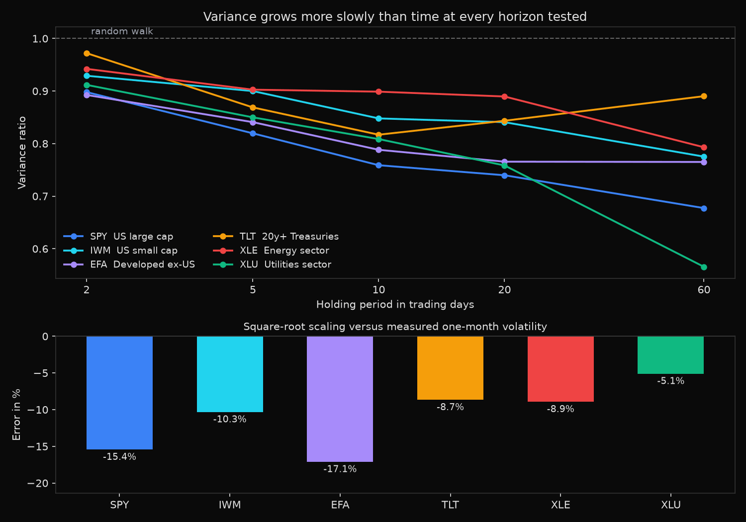
Variance ratio test on daily total returns, 2006-01-03 to 2025-12-31
Overlapping estimator, heteroskedasticity-robust z (Lo and MacKinlay 1988)
VR = 1 means variance grows linearly with time; * marks |z| > 1.96

         obs  ann vol             q=2             q=5            q=10            q=20            q=60
                           VR       z      VR       z      VR       z      VR       z      VR       z
SPY     5031   19.4%   0.898  -3.09*   0.820  -2.33*   0.759  -2.05*   0.740  -1.56    0.677  -1.24
IWM     5031   24.6%   0.929  -2.67*   0.900  -1.63    0.848  -1.62    0.841  -1.20    0.775  -1.05
EFA     5031   21.5%   0.893  -3.42*   0.841  -2.18*   0.788  -1.90    0.766  -1.46    0.765  -0.91
TLT     5031   14.9%   0.972  -1.13    0.869  -2.53*   0.817  -2.37*   0.843  -1.47    0.890  -0.66
XLE     5031   30.3%   0.942  -2.08*   0.903  -1.46    0.899  -0.95    0.890  -0.72    0.793  -0.85
XLU     5031   18.8%   0.912  -2.36*   0.850  -1.78    0.809  -1.49    0.758  -1.34    0.566  -1.61

What the square-root rule costs at a one-month horizon
                          20-day sd  sqrt(20) x daily    error  blocks
SPY   US large cap           4.62%            5.47%   -15.4%     251
IWM   US small cap           6.21%            6.92%   -10.3%     251
EFA   Developed ex-US        5.01%            6.05%   -17.1%     251
TLT   20y+ Treasuries        3.83%            4.19%    -8.7%     251
XLE   Energy sector          7.76%            8.52%    -8.9%     251
XLU   Utilities sector       5.04%            5.31%    -5.1%     251

Rows removed by the return-bound screen: 0
Implied one-month volatility from VR(20), annualised:
  SPY    19.4% naive     16.7% VR-adjusted
  IWM    24.6% naive     22.5% VR-adjusted
  EFA    21.5% naive     18.8% VR-adjusted
  TLT    14.9% naive     13.7% VR-adjusted
  XLE    30.3% naive     28.5% VR-adjusted
  XLU    18.8% naive     16.4% VR-adjusted

What this tells us

Every one of the thirty variance ratios sits below 1. Variance grew more slowly than time for all six funds at all five horizons, the signature of negative serial correlation rather than a random walk.

At two days the departure is statistically solid, five of the six rejecting at 5 percent and EFA strongest at z = -3.42. VR(2) minus 1 is exactly the first-order autocorrelation of daily returns, so SPY’s 0.898 says its returns carried an autocorrelation of -0.102. TLT is the exception at 0.972.

Point estimates keep sliding as the horizon lengthens, SPY reaching 0.740 at twenty days and XLU 0.566 at sixty, yet the z statistics move the other way. Nothing rejects at twenty or sixty days, the largest value being XLU at -1.61. The cause is arithmetic: twenty years holds 251 independent 20-day blocks and 83 independent 60-day blocks, so the standard error widens faster than the estimate falls. SPY’s VR(20) of 0.740 carries a standard error of 0.167 and a 95 percent interval of 0.41 to 1.07, which fails to exclude 1.

The block check agrees everywhere: measured one-month standard deviation came in below the square-root-scaled figure for all six funds, by 5.1 percent for XLU and 17.1 percent for EFA. Magnitudes differ because 251 blocks is thin, but the direction is unanimous.

So what?

The square-root rule overstated multi-day risk on all six funds, and overstatement is the forgiving direction for a risk limit. Nobody needs to stop multiplying by the square root of 252.

The bias bites when a scaled figure meets a market quote. One-month implied volatility against annualised daily realised volatility is not like for like: the realised leg carried an upward bias between 5.7 percent for XLE and 14.0 percent for SPY, so SPY’s naive 19.4 percent becomes 16.7 percent once VR(20) is applied. A variance risk premium computed without that adjustment reads wider than it is.

For anyone trading the pattern rather than measuring it, the two-day result is the only firm finding here, and an autocorrelation of -0.10 on SPY sits below the round-trip cost most participants pay. The longer-horizon ratios are unproven, and trading them needs more data than twenty years supplies.

Test the specific asset at the specific horizon before scaling, and read the ratio next to its standard error rather than alone.

Built with xfinlink — free financial data API for Python. pip install -U xfinlink