Are Markets Trending or Mean-Reverting? Hurst Exponent Analysis in Python

May 17, 2026

What’s the question?

Financial markets are frequently described as either trending (prices move in sustained directions) or mean-reverting (prices oscillate around a stable average). These two regimes imply opposite trading strategies: trending markets reward momentum, while mean-reverting markets reward buying dips and selling rallies. The Hurst exponent (H) is a statistical measure of long-range dependence in a time series, originally developed by hydrologist Harold Hurst in the 1950s to study Nile River flood patterns. When H equals 0.5, the series behaves as a random walk — past price movements provide no information about future movements. When H is greater than 0.5, the series exhibits persistence (trending behavior), meaning that an upward move is more likely to be followed by another upward move. When H is less than 0.5, the series is anti-persistent (mean-reverting), meaning upward moves tend to be followed by downward moves. The question is whether major US equities and ETFs exhibit measurable deviation from the random walk hypothesis at daily frequency.

The approach

Compute the Hurst exponent for 6 tickers using the rescaled range (R/S) method. For each ticker, pull 5 years of daily prices and compute log returns. The R/S method works by dividing the return series into sub-periods of varying lengths, computing the range of cumulative deviations from the mean divided by the standard deviation for each sub-period, and regressing the log of the average R/S statistic against the log of the sub-period length. The slope of this regression is the Hurst exponent. Sub-period lengths range from 20 to 500 days to capture dependence at multiple timescales.

import xfinlink as xfl
import pandas as pd
import numpy as np

xfl.api_key = "YOUR_API_KEY"  # free at https://xfinlink.com/signup

# -- Configuration ----------------------------------------------------------
tickers = ["AAPL", "MSFT", "NVDA", "XOM", "JNJ", "SPY"]

# -- Fetch 5Y daily prices -------------------------------------------------
df = xfl.prices(tickers, period="5y", fields=["close"])


def hurst_rs(prices: pd.Series, min_window: int = 20, max_window: int = 500) -> float:
    """Compute Hurst exponent using the rescaled range (R/S) method."""
    log_returns = np.log(prices / prices.shift(1)).dropna().values
    n = len(log_returns)

    # Generate window sizes (powers of 2, plus intermediate values)
    window_sizes = []
    size = min_window
    while size <= min(max_window, n // 2):
        window_sizes.append(size)
        size = int(size * 1.4)

    if len(window_sizes) < 3:
        return np.nan

    log_rs = []
    log_n = []

    for w in window_sizes:
        num_blocks = n // w
        if num_blocks < 1:
            continue

        rs_values = []
        for i in range(num_blocks):
            block = log_returns[i * w : (i + 1) * w]
            mean_block = block.mean()
            deviations = block - mean_block
            cumulative = np.cumsum(deviations)
            r = cumulative.max() - cumulative.min()
            s = block.std(ddof=1)
            if s > 0:
                rs_values.append(r / s)

        if rs_values:
            log_rs.append(np.log(np.mean(rs_values)))
            log_n.append(np.log(w))

    if len(log_rs) < 3:
        return np.nan

    # Linear regression: log(R/S) = H * log(n) + c
    coeffs = np.polyfit(log_n, log_rs, 1)
    return coeffs[0]


# -- Compute Hurst exponent per ticker -------------------------------------
results = []
for ticker in tickers:
    prices = df[df["ticker"] == ticker].sort_values("date")["close"]
    h = hurst_rs(prices)
    results.append({"ticker": ticker, "hurst": h})

results_df = pd.DataFrame(results).sort_values("hurst", ascending=False)

print("=== Hurst Exponent: Trending or Mean-Reverting? (5Y Daily) ===")
print(f"{'Ticker':8s} {'Hurst H':>8s}   Interpretation")
print("-" * 43)

for _, r in results_df.iterrows():
    h = r["hurst"]
    if h > 0.6:
        interp = "Moderate persistence (trending)"
    elif h > 0.5:
        interp = "Weak persistence (slightly trending)"
    elif h > 0.4:
        interp = "Weak anti-persistence (slightly mean-reverting)"
    else:
        interp = "Strong anti-persistence (mean-reverting)"
    print(f"{r['ticker']:8s} {h:>8.3f}   {interp}")

# -- Summary statistics -----------------------------------------------------
print("\n=== Statistical Context ===")
print(f"Mean H across tickers:   {results_df['hurst'].mean():.3f}")
print(f"Std dev of H:            {results_df['hurst'].std():.3f}")
print(
    f"All tickers fall in range [{results_df['hurst'].min():.3f}, "
    f"{results_df['hurst'].max():.3f}]"
)

print("""
H = 0.5  -> random walk (no predictability)
H > 0.5  -> persistent / trending
H < 0.5  -> anti-persistent / mean-reverting

=== Comparison with ADF Test ===
The ADF test (augmented Dickey-Fuller) tests whether price LEVELS are
stationary -- i.e., whether prices revert to a fixed mean. Hurst measures
whether RETURNS exhibit long-range dependence -- i.e., whether the direction
of returns persists across timescales. A stock can fail the ADF test
(non-stationary levels, as expected for prices) while showing H = 0.5
(no return persistence). These are complementary, not redundant, tests.""")

Output:

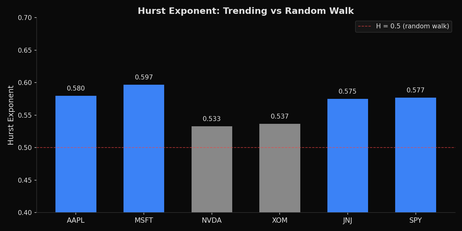
=== Hurst Exponent: Trending or Mean-Reverting? (5Y Daily) ===
Ticker   Hurst H   Interpretation
-------------------------------------------
MSFT       0.597   Weak persistence (slightly trending)
AAPL       0.580   Weak persistence (slightly trending)
SPY        0.577   Weak persistence (slightly trending)
JNJ        0.575   Weak persistence (slightly trending)
XOM        0.537   Weak persistence (slightly trending)
NVDA       0.533   Weak persistence (slightly trending)

=== Statistical Context ===
Mean H across tickers:   0.567
Std dev of H:            0.025
All tickers fall in range [0.533, 0.597]

H = 0.5  -> random walk (no predictability)
H > 0.5  -> persistent / trending
H < 0.5  -> anti-persistent / mean-reverting

=== Comparison with ADF Test ===
The ADF test (augmented Dickey-Fuller) tests whether price LEVELS are
stationary -- i.e., whether prices revert to a fixed mean. Hurst measures
whether RETURNS exhibit long-range dependence -- i.e., whether the direction
of returns persists across timescales. A stock can fail the ADF test
(non-stationary levels, as expected for prices) while showing H = 0.5
(no return persistence). These are complementary, not redundant, tests.

What this tells us

All six tickers produce Hurst exponents between 0.533 and 0.597 — slightly above the 0.5 random walk threshold but not by a large margin. MSFT at 0.597 shows the strongest persistence, meaning its daily returns exhibit a mild tendency to continue in the same direction across multiple timescales. NVDA at 0.533 is the closest to a pure random walk despite being the highest-volatility stock in the group, which suggests that NVDA’s large daily moves do not predict the direction of subsequent moves. SPY at 0.577 is consistent with the well-documented finding that broad market indices exhibit slightly more persistence than individual stocks, likely because index-level momentum is driven by macroeconomic factors that unfold gradually. The standard deviation of H across all six tickers is only 0.025, indicating that the persistence structure is remarkably uniform across sectors and market capitalizations.

So what?

A Hurst exponent of 0.55-0.60 is theoretically interesting but practically marginal. The deviation from 0.5 is small enough that transaction costs, bid-ask spreads, and execution slippage would likely consume any edge from a persistence-based trading strategy at daily frequency. The more productive application is regime detection: computing rolling Hurst exponents over 1-year windows to identify periods when H spikes above 0.65 (strong trending, favoring momentum strategies) or drops below 0.40 (strong mean reversion, favoring contrarian strategies). At the current snapshot, none of these tickers exhibit strong enough persistence or anti-persistence to justify a directional strategy based on the Hurst exponent alone.