Does Cointegration Survive Out of Sample? Pairs Trading Validation in Python

August 5, 2026

What’s the question?

Pairs trading rests on cointegration. Two share prices can each wander with no fixed level to return to, and yet one combination of them stays anchored: the gap opens, closes, opens again. Engle and Granger set out the standard test in 1987. Regress one log price on the other and test the residual for a unit root; a p-value below 0.05 says the spread is stationary, which is the licence a mean-reversion rule needs.

The test looks backwards and the trade happens afterwards. Nothing promises that a relationship measured over three years is still there in the fourth. Worse, at the 5% level a test rejects a true unit root one time in twenty by construction, so a thousand-pair screen produces about fifty passes from noise alone.

The question is therefore not whether same-industry pairs pass the test. It is whether passing says anything about the three years that follow.

The approach

1. Take S&P 500 members as at 5 August 2020, keyed on entity identifiers rather than symbols, so companies that later left the index stay in the sample.
2. Map each member to its GICS industry and keep the ten industries with the most members.
3. Pull daily split-adjusted closes from 5 August 2020 to 4 August 2026. Names that traded under more than one symbol in the window, and names without a complete daily history for it, leave the panel: 148 companies and 1,506 sessions remain.
4. Split the window in half: 755 formation sessions ending 4 August 2023, 751 holdout sessions after it. Test all 1,048 within-industry pairs once in each window, estimated independently, with the regression direction fixed alphabetically since Engle-Granger is not symmetric.
5. Freeze the formation hedge ratio, spread mean and spread standard deviation, then run the textbook entry rule forward: open when the z-score of the spread reaches plus or minus 2, close when it returns to zero, abandon after 60 sessions.

One detail decides whether the p-values mean anything. The series tested is a fitted residual, not an observed one, so the ordinary Dickey-Fuller distribution is too generous and the Engle-Granger critical values from MacKinnon are the correct reference; statsmodels.tsa.stattools.coint applies them. Marathon Petroleum against ExxonMobil gives the same statistic either way, −3.705, and p = 0.018 against the correct table where the ordinary one reads 0.0002.

Code

import itertools
import numpy as np
import pandas as pd
import xfinlink as xfl
from statsmodels.regression.linear_model import OLS
from statsmodels.tools import add_constant
from statsmodels.tsa.stattools import coint

xfl.set_api_key("YOUR_API_KEY")  # free at https://xfinlink.com/signup

FORM_END = "2023-08-04"

members = xfl.index("sp500", as_of="2020-08-05").dropna(subset=["entity_id"])
ids = sorted(members["entity_id"].astype(int))
px = pd.concat([xfl.prices(entity_id=ids[i:i + 5], start="2020-08-05", end="2026-08-04",
                           fields=["adj_close"], max_rows=200000)
                for i in range(0, len(ids), 5)], ignore_index=True)
# uni carries the GICS industry of each entity from xfl.resolve(); sym maps id to symbol

wide = px.pivot_table(index="date", columns="entity_id", values="adj_close").sort_index()
form, hold = wide.loc[:FORM_END], wide.loc[wide.index > FORM_END]
keep = [i for i in wide.columns
        if form[i].notna().all() and hold[i].notna().all() and wide[i].min() > 0]
lf, lh = np.log(form[keep]), np.log(hold[keep])

for industry, grp in uni.groupby("industry"):
    for a, b in itertools.combinations(sorted(grp["entity_id"], key=lambda e: sym[e]), 2):
        p_form = coint(lf[b].values, lf[a].values, trend="c", autolag="AIC")[1]
        p_hold = coint(lh[b].values, lh[a].values, trend="c", autolag="AIC")[1]

        fit = OLS(lf[b].values, add_constant(lf[a].values)).fit()
        z = (lh[b].values - fit.params[0] - fit.params[1] * lh[a].values
             - fit.resid.mean()) / fit.resid.std(ddof=1)

        print(f"{sym[a]}/{sym[b]}: formation p={p_form:.4f}  holdout p={p_hold:.4f}  "
              f"holdout entries={(np.abs(z) >= 2).sum()}")

Full script with formatting and visualisation: cointegration-out-of-sample-pairs-python.py

Output

Panel: 148 names, 1048 same-industry pairs, 755 formation sessions, 751 holdout sessions
Formation cointegrated at 5%: 49 (4.68%), chance alone predicts 52.4
Holdout cointegrated at 5%:   62 (5.92%)
Repeat rate, selected pairs:  1/49 (2.0%)
Repeat rate, rejected pairs:  61/999 (6.1%)
At the 1% level: 7 selected, 0 repeat

Holdout entry rule: enter at |z| >= 2, exit at z = 0 or after 60 sessions
group          trades  converged  median days  mean sigma  mean log ret
selected          185      18.9%           39      -0.119        -0.52%
rejected         2716       6.7%           38       0.010         0.13%
  converged trades: mean +2.34 sigma
  timed out trades: mean -0.19 sigma

What this tells us

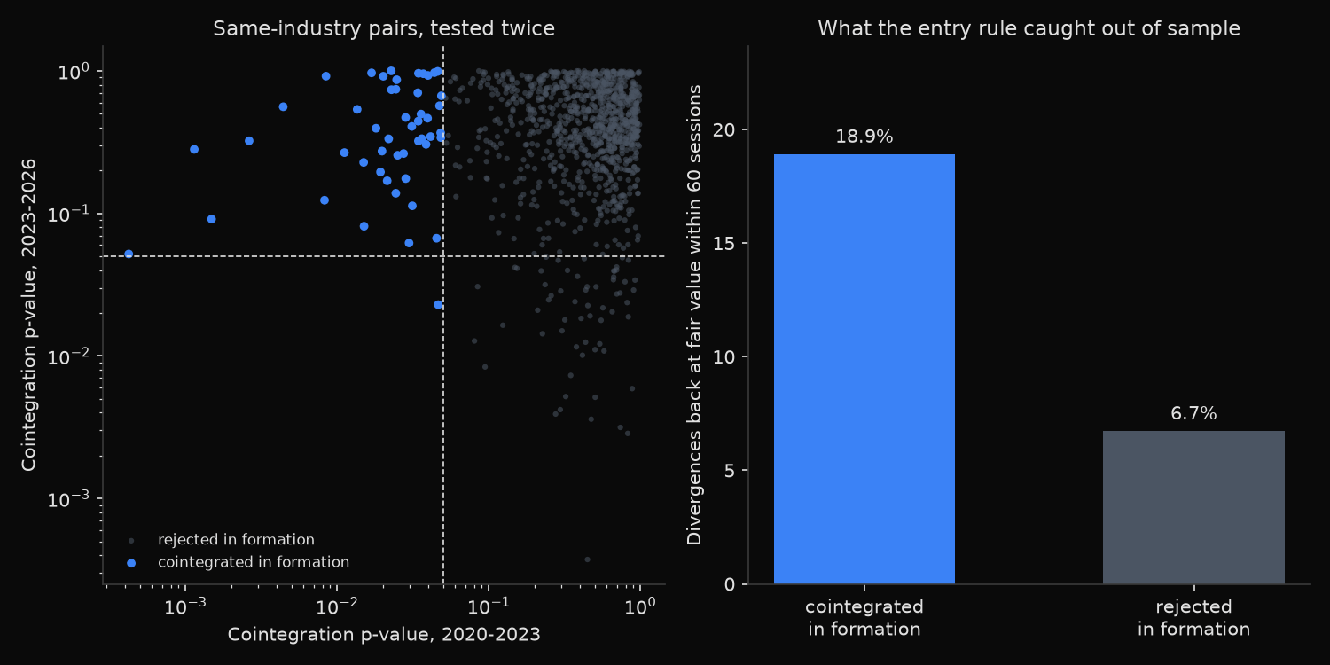
The formation screen found nothing that chance would not have produced. 49 of 1,048 pairs cleared the 5% threshold against 52.4 expected when no pair is cointegrated at all, and tightening to 1% leaves 7 against 10.5 expected. At this sample size the count of cointegrated peers in a sector screen restates the significance level.

Repetition is where the case collapses. One of the 49 selected pairs passed again in the holdout, a repeat rate of 2.0%, against 6.1% for the 999 pairs the screen rejected. Selection did not raise the odds of a stationary spread over the next three years, and a Fisher exact test returns p = 0.36, so even that reversal is noise. None of the 7 pairs selected at the 1% level repeated.

The entry rule tells a subtler story. Divergences on the selected pairs came back to fair value within 60 sessions 18.9% of the time against 6.7% for the rejected pairs, so the formation test carried real information about short-horizon convergence even where it carried none about cointegration. The outcome does not follow. A converged trade returns +2.34 standard deviations of spread and a stalled one loses 0.19, and the stalled trades on selected pairs run further than that: the selected book averages −0.119 standard deviations per entry, or −0.52% in log terms, against +0.010 for the rejected book. A few episodes dominate, with the MPC/XOM spread alone giving back 10.3 standard deviations. Trim outcomes at plus or minus 3 and both books sit at zero.

So what?

Count the tests before trusting any of them. A screen of 1,048 pairs at the 5% level turns noise into 52 candidates, and the correction costs one line: divide the threshold by the number of tests. At 0.05/1048 the strongest p-value in this panel is BDX against STE at 0.00042, nine times too large to pass. Not one same-industry pair clears a multiple-testing correction over these three years.

The stronger discipline is a holdout: fit the hedge ratio on one window, then require the relationship to hold on a later window that took no part in the fitting before any capital moves. Pairs that pass twice are rare, and that scarcity is the signal about how many deserve a position.

For a book already running, the asymmetry is what to size against. Winners come home in about 39 sessions and pay roughly two and a third standard deviations; losers keep going. An entry band without exit discipline is short that left tail, and a cointegration test at entry does nothing to shorten it.

Built with xfinlink — free financial data API for Python. pip install -U xfinlink