
Which Volatility Forecast Wins One Month Ahead? HAR vs EWMA in Python
July 29, 2026
What's the question?
Position sizing, option pricing and risk limits all need a number for how volatile an asset will be over some future window. The common shortcut is the last month of daily returns: take their standard deviation and annualise it. Realized volatility here means the square root of 252 times the average squared daily log return over a window, so a reading of 15 is a 15% annualised standard deviation.
Carrying that trailing figure forward treats volatility as a random walk. Volatility is persistent, so the assumption captures something real, but it also reverts: quiet periods drift up toward the long-run average and panics decay back down. A forecast anchored on the most recent month inherits every shock at full strength.
Two standard models try to do better. Exponentially weighted moving average, the RiskMetrics convention, decays squared returns geometrically at 0.94, so recent days dominate without a hard window cutoff. The heterogeneous autoregressive model of Fulvio Corsi (2009) instead regresses future volatility on realized volatility measured over three horizons at once, since participants trade on different clocks.
The approach
Six liquid names from July 2005 to June 2026, spanning a wide volatility range: SPY and IWM for large and small cap indices, AAPL and MSFT, JPM through two banking crises, and KO at the quiet end. Returns are log changes in split-adjusted closes.
- Compute annualised realized volatility over the trailing 5, 21 and 63 trading days.
- Set the target to realized volatility over the following 21 trading days, starting the day after the forecast is made.
- Fit HAR by ordinary least squares of the target on the three trailing measures.
- Benchmark against the trailing 21-day figure carried forward, the RiskMetrics estimate, and the expanding-window average of the target.
- Start forecasting in January 2016, refitting at each test point on all data whose target windows close before that day.
- Evaluate every 21st trading day only: 125 non-overlapping windows per name, 750 in total.
The last two steps matter more than the model choice. Overlapping monthly windows share 20 of their 21 days, so scoring on them inflates the apparent sample size roughly twentyfold. One squared daily return is too noisy to stand alone, so the shortest component here is a week rather than Corsi’s intraday daily term.
Code
import numpy as np
import pandas as pd
import xfinlink as xfl

xfl.set_api_key("YOUR_API_KEY")  # free at https://xfinlink.com/signup

TICKERS = ["SPY", "IWM", "AAPL", "MSFT", "JPM", "KO"]
H, LAM = 21, 0.94

px = pd.concat([xfl.prices(t, start="2005-07-01", end="2026-06-30",
                           fields=["adj_close"]) for t in TICKERS],
               ignore_index=True)

def panel(ticker):
    s = px[px["ticker"] == ticker].sort_values("date").set_index("date")
    sq = np.log(s["adj_close"]).diff().pow(2)
    av = lambda w: np.sqrt(252.0 * sq.rolling(w).mean())
    fwd = sq[::-1].rolling(H).mean()[::-1].shift(-1)   # days t+1 .. t+H
    return pd.DataFrame({
        "v5": av(5), "v21": av(21), "v63": av(63),
        "ewma": np.sqrt(252.0 * sq.ewm(alpha=1 - LAM, adjust=False).mean()),
        "y": np.sqrt(252.0 * fwd)}).dropna()

def fit(X, y):
    return np.linalg.lstsq(np.column_stack([np.ones(len(X)), X]), y, rcond=None)[0]

COLS = ["v5", "v21", "v63"]
for t in TICKERS:
    d = panel(t)
    recs = []
    for i in np.flatnonzero(d.index >= "2016-01-01")[::H]:
        train = d.iloc[:i - H]          # last training target ends before day i
        b = fit(train[COLS].values, train["y"].values)
        recs.append({"actual": d.iloc[i]["y"], "rw": d.iloc[i]["v21"],
                     "ewma": d.iloc[i]["ewma"],
                     "har": float(b[0] + b[1:] @ d.iloc[i][COLS].values)})
    e = pd.DataFrame(recs)
    rmse = {m: np.sqrt(((e[m] - e["actual"]) ** 2).mean()) for m in ["har", "ewma", "rw"]}
    print(t, {k: round(v * 100, 2) for k, v in rmse.items()})
Full script with formatting and visualisation: volatility-forecast-har-vs-ewma-python.py
Output
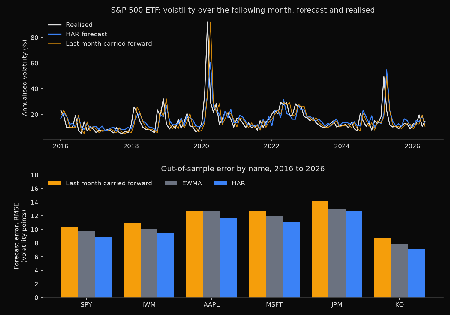
Out-of-sample monthly volatility forecasts, 2016-01-04 to 2026-05-13  (750 non-overlapping windows)

           mean vol   RMSE, annualised volatility points      HAR gain
                        HAR    EWMA      RW    mean   vs RW
   SPY       14.9    8.87    9.77   10.31   10.13    26.1%
   IWM       20.5    9.48   10.13   10.98   10.67    25.4%
  AAPL       26.1   11.63   12.70   12.79   13.04    17.3%
  MSFT       24.3   11.07   11.91   12.61   12.04    22.9%
   JPM       23.8   12.68   12.95   14.18   15.32    20.1%
    KO       16.1    7.14    7.86    8.74    8.68    33.2%
pooled       20.9   10.31   11.04   11.74   11.84    22.8%

Mean forecast error (forecast minus realised, volatility points)
  calm months      n=375   HAR  +0.17   EWMA  -1.37   RW  -2.67
  stressed months  n=375   HAR  +1.04   EWMA  +2.51   RW  +2.64

Final HAR coefficients (intercept, week, month, quarter)
     SPY   0.051   0.401   0.204   0.093   slope sum 0.698
     IWM   0.063   0.293   0.298   0.125   slope sum 0.716
    AAPL   0.109   0.202   0.212   0.209   slope sum 0.623
    MSFT   0.090   0.175   0.160   0.299   slope sum 0.634
     JPM   0.049   0.192   0.182   0.453   slope sum 0.827
      KO   0.059   0.270   0.092   0.281   slope sum 0.643

SPY through the 2020 shock
        date   realised      HAR       RW
  2020-01-06      13.1%    10.4%     7.5%
  2020-02-05      35.1%    15.7%    13.1%
  2020-03-06      92.1%    36.1%    35.1%
  2020-04-06      29.4%    60.6%    92.1%
  2020-05-06      21.7%    25.9%    29.4%
  2020-06-05      28.3%    23.4%    21.7%
What this tells us
HAR produces the lowest error on all six names, and the ordering never changes: HAR, then EWMA, then the trailing month, with the long-run average last or near it. Pooled across 750 windows the error falls from 11.74 volatility points to 10.31, a 22.8% cut in mean squared error, 33.2% for KO down to 17.3% for AAPL.
The bias table shows where that comes from. In calm months the trailing-month rule under-forecasts by 2.67 volatility points; in stressed months it over-forecasts by 2.64. The sign flips because carrying the current level forward gives no weight to the pull toward the long-run mean. EWMA halves the calm-month error and keeps almost all of the stressed-month one. HAR misses by 0.17 points in calm months and 1.04 in stressed ones.
The coefficients show the mechanism. Every slope sum lands between 0.62 and 0.83, so the forecast shrinks toward the intercept rather than tracking the current level one for one; the mean reversion is estimated, not assumed. Horizon weights differ by name, SPY putting 0.40 on the week against 0.09 on the quarter while JPM puts 0.45 on the quarter, so one fixed weighting for every asset gives back part of the gain.
March 2020 marks the limit of the exercise. From information ending 6 March, HAR forecast 36.1% against a realized 92.1%. The advantage lands on the far side of the spike: on 6 April the trailing-month rule carried 92.1% into a month that realized 29.4%, while HAR called 60.6%.
So what?
Anyone sizing positions off a trailing 21-day volatility estimate carries a known, signed error. The estimate runs low in quiet markets, so exposure peaks exactly when a shock would hurt most, and runs high afterward, keeping exposure suppressed through the recovery. That is the reverse of what the sizing rule was meant to do.
The fix is three columns and one regression: realized volatility over a week, a month and a quarter, regressed on the next month’s realized volatility and refit as data arrives. Fit it per asset, because the horizon weights are not stable across names. Where that is more machinery than a desk wants, shrinking the trailing estimate roughly 30% of the way toward the asset’s own long-run average removes most of the sign-flipping bias.
What should not survive is the evaluation shortcut. Scoring a monthly forecast on overlapping daily windows counts each month about twenty times, and will make almost any model look significant.
pip install -U xfinlink