
How Many Stocks Does It Take to Diversify? Random Portfolio Simulation in Python
August 4, 2026
What’s the question?
A concentrated equity manager holds 25 to 30 names and cites the standard result: past roughly 30 stocks, the volatility saved by adding another is too small to matter. Evans and Archer put the number near 10 in 1968, and Statman revised it upward in 1987, to at least 30 for a borrowing investor and 40 for a lending one.
Every version of that result describes an average. Draw many 30-stock portfolios at random, measure the volatility of each, and the mean sits close to the volatility of the market itself.
Nobody holds the average portfolio. An investor holds one draw from a distribution, and the width of that distribution is itself a risk. Both the typical risk of an N-name portfolio and the spread of risk across the portfolios that could have been picked instead shrink as N grows, at different speeds, and the second is the one a risk budget has to survive.
The approach
The exercise draws random equal-weighted portfolios from S&P 500 members and measures two properties of each: annualised volatility, and maximum drawdown, the deepest fall from a running peak of the cumulative return path.
- Take the current index roster, keyed on entity identifiers.
- Pull daily split-adjusted closes from 4 August 2021 to 3 August 2026. Set aside entities that traded under more than one symbol in the window, names without a complete daily history, and any name whose largest single-day change exceeds 100%, a size that records a corporate action rather than a price change. 435 companies and 1,253 sessions survive.
- For each portfolio size from 1 to 100, draw 2,000 random subsets without replacement, equally weighted and rebalanced daily so the weights stay fixed.
- Report the mean and the 10th and 90th percentiles of each measure across the draws.
Fixed weights buy a closed form worth checking against. Expected variance for N names drawn at random equals the average single-name variance divided by N, plus the average pairwise covariance multiplied by (1 − 1/N). The first term is what diversification removes; the second is a floor that does not move. The roster is current membership, so the panel holds index members as at the end of the window; the measures reported depend on the covariance structure rather than on average returns.
Code
import numpy as np
import pandas as pd
import xfinlink as xfl

xfl.set_api_key("YOUR_API_KEY")  # free at https://xfinlink.com/signup

SIZES = [1, 2, 3, 5, 8, 10, 15, 20, 25, 30, 40, 50, 75, 100]
DRAWS, SEED = 2000, 20260804

members = xfl.index("sp500").dropna(subset=["entity_id"])
ids = sorted(set(members["entity_id"].astype(int)))
px = pd.concat([xfl.prices(entity_id=ids[i:i + 100], start="2021-08-04",
                           end="2026-08-03", fields=["adj_close"], max_rows=200000)
                for i in range(0, len(ids), 100)], ignore_index=True)

single = px.groupby("entity_id")["ticker"].nunique() == 1
wide = (px[px["entity_id"].isin(single[single].index)]
        .pivot_table(index="date", columns="ticker", values="adj_close").sort_index())
ret = wide.dropna(axis=1).pct_change().dropna()
ret = ret.drop(columns=ret.columns[ret.abs().max() >= 1.0])


def max_dd(r):
    curve = (1.0 + r).cumprod()
    return float((curve / np.maximum.accumulate(curve) - 1.0).min())


R = ret.to_numpy()
rng = np.random.default_rng(SEED)
for n in SIZES:
    vol, dd = [], []
    for _ in range(DRAWS):
        p = R[:, rng.choice(R.shape[1], size=n, replace=False)].mean(axis=1)
        vol.append(p.std(ddof=1) * np.sqrt(252))
        dd.append(max_dd(p))
    print("%4d  volatility mean %.2f unlucky %.2f   drawdown mean %.2f unlucky %.2f"
          % (n, 100 * np.mean(vol), 100 * np.percentile(vol, 90),
             100 * np.mean(dd), 100 * np.percentile(dd, 10)))

S = np.cov(R, rowvar=False, ddof=1)
avg_var, avg_cov = np.mean(np.diag(S)), S[~np.eye(len(S), dtype=bool)].mean()
print("systematic floor %.2f" % (100 * np.sqrt(avg_cov * 252)))
Full script with formatting and visualisation: how-many-stocks-to-diversify-python.py
Output
S&P 500 members, daily returns from split-adjusted closes
2021-08-05 to 2026-08-03 (1,253 sessions)
503 roster entities, 477 under a single symbol across the window,
436 with a complete daily history, 435 in the panel after the corporate-action screen

Equal-weighted portfolios rebalanced daily, 2,000 random draws per size

            annualised volatility %        maximum drawdown %
  size     mean   lucky   unlucky        mean   lucky   unlucky
     1    32.00   21.41    45.97      -46.37  -27.16    -67.64
     2    25.89   19.26    34.24      -37.19  -23.70    -53.64
     3    23.31   18.20    29.30      -32.79  -21.80    -45.49
     5    20.73   16.90    25.04      -27.93  -19.51    -37.69
     8    19.21   16.34    22.55      -25.53  -18.85    -33.08
    10    18.79   16.11    21.77      -24.67  -18.50    -31.76
    15    17.93   15.87    20.13      -23.23  -18.29    -28.84
    20    17.64   15.83    19.56      -22.78  -18.26    -27.59
    25    17.37   15.78    19.07      -22.24  -18.33    -26.63
    30    17.22   15.77    18.75      -21.97  -18.22    -25.99
    40    16.98   15.74    18.33      -21.54  -18.30    -25.24
    50    16.92   15.78    18.09      -21.41  -18.42    -24.61
    75    16.72   15.87    17.58      -20.94  -18.54    -23.48
   100    16.65   15.94    17.40      -20.74  -18.70    -22.90
   all    16.45                      -20.20

  lucky = 10th percentile of the 2,000 draws, unlucky = 90th

Systematic floor from average pairwise covariance   16.39%
SPY over the same window: volatility 17.24%, maximum drawdown -25.36%

Simulated against closed form, annualised volatility
  size   simulated   closed form   difference bp
     1       33.78         33.78           -0.9
     2       26.68         26.55          +12.6
     3       23.77         23.65          +11.5
     5       20.99         21.05           -6.2
     8       19.37         19.43           -6.6
    10       18.92         18.86           +6.3
    15       18.01         18.07           -5.9
    20       17.70         17.67           +3.0
    25       17.42         17.42           -0.3
    30       17.26         17.25           +0.8
    40       17.01         17.04           -2.6
    50       16.94         16.91           +3.4
    75       16.74         16.74           +0.1
   100       16.66         16.65           +1.1
What this tells us
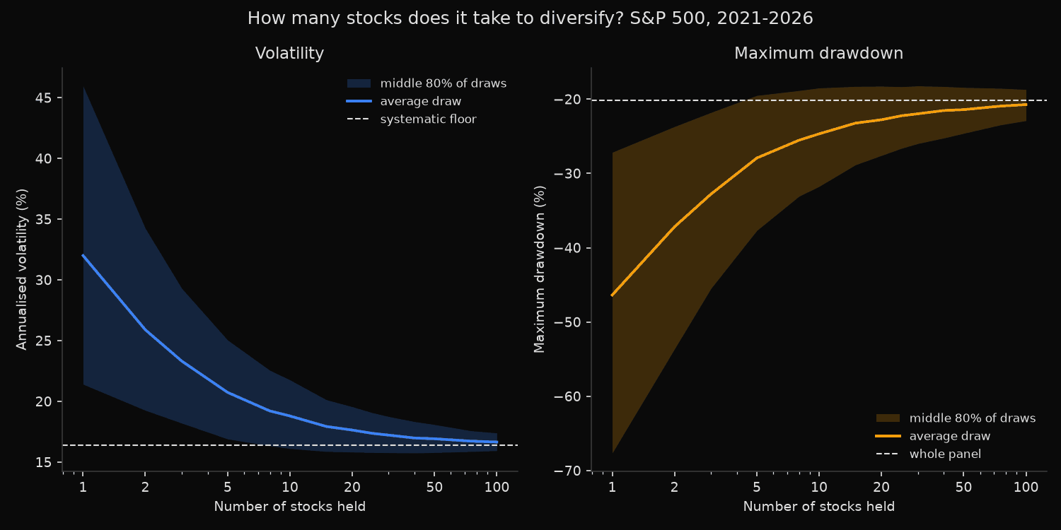
The average curve reproduces the textbook. A single stock averaged 32.00% annualised volatility, ten names 18.79%, thirty names 17.22%, and the whole 435-name panel 16.45%. The floor implied by average pairwise covariance is 16.39%, so the average 30-stock portfolio sits within 0.83 points of a limit it cannot cross, and the remaining 405 names buy that 0.83 between them. Simulation and closed form agree to within 13 basis points at every size, confirming the simulation measures the quantity the algebra describes.
The percentiles carry the other half. At 30 names the average draw carried 17.22% volatility and the unlucky decile carried 18.75%, which is 2.36 points above the floor rather than 0.83. Pushing the unlucky decile down to where the average 20-stock portfolio already sits takes about 75 names: 17.58% against 17.64%. The average converges roughly four times faster than the tail.
Drawdown separates them further. The whole panel fell 20.20% at worst and SPY, which is capitalisation-weighted, fell 25.36%. The average 30-stock portfolio fell 21.97%; the unlucky decile fell 25.99%, deeper than the tracker.
The shallow end stops improving early. Between 8 names and 100 the shallowest decile of drawdowns travels from 18.85% to 18.70%, no movement at all, while the deep end improves across that whole range, from 33.08% to 22.90%. Names added after the first handful buy protection against the bad draw and little else.
So what?
A mandate capped at 25 or 30 holdings is not a mandate to accept much more volatility: on average it costs about a point against a 400-name basket. What it accepts is uncertainty over which 30, and one portfolio in ten built that way carried a drawdown 5.8 points deeper than the panel over a window whose worst stretch was the 2022 decline.
Size the risk budget off the unlucky percentile rather than the average: for a 30-name book in this market, plan around a 26% drawdown, not 22%. Then treat every marginal-name decision as a question about that tail. Moving from 30 holdings to 50 shifts average volatility by 0.30 points, the unlucky decile of volatility by 0.66, and the unlucky decile of drawdown by 1.38. The case for concentration is normally argued on the average — the bill arrives in the tail.
Built with xfinlink — free financial data API for Python. pip install -U xfinlink
pip install -U xfinlink