
What’s the question?
Two numbers describe an equity market over a year, and they are routinely treated as one. Volatility measures how sharply the index moves from day to day. Dispersion measures how far apart its members finish from each other over the same window: the standard deviation of member returns taken across the index at a point in time rather than through time.
Dispersion sets the size of the prize in stock selection. If every member lands within a few points of the average, correct picks cannot add much and wrong picks cannot cost much; when the members finish a hundred points apart, the same amount of skill produces a far larger result in either direction.
Market commentary tends to assume the two travel together, and that a turbulent market rewards selection. That assumption is testable, along with the related idea that a violent year hands the next one a wide cross-section.
The approach
The sample is the 20 calendar years from 2006 to 2025.
- Rebuild S&P 500 membership on the first day of each year from the roster as it stood on that date, carrying every member by company identifier rather than ticker, so a company removed later still counts for the years it was a member.
- Pull daily total returns for each member and compound them into a full-year return inside the script, which keeps a company that changes its symbol mid-year intact.
- Apply two screens: a member needs a price series covering at least 95 percent of the year’s trading days, and its daily returns have to agree with its own price path day by day.
- Compute dispersion as the standard deviation of those annual returns across members, and the decile spread as the average return of the best tenth minus the average of the worst tenth.
- Measure the index itself over the same years through SPY, using annualised daily volatility.
That yields 9,532 member-years, between 443 and 495 members per year.
Code
import time
import numpy as np
import pandas as pd
from scipy import stats
import xfinlink as xfl

xfl.set_api_key("YOUR_API_KEY")  # free at https://xfinlink.com/signup

YEARS = list(range(2006, 2026))
CHUNK = 50


def fetch(**kwargs):
    for attempt in range(5):
        try:
            return xfl.prices(**kwargs)
        except xfl.XfinlinkError as exc:
            last = exc
            time.sleep(4 * (attempt + 1))
    raise last


rows = []
for year in YEARS:
    roster = xfl.index("sp500", as_of=f"{year}-01-01")
    ids = sorted({int(e) for e in roster["entity_id"].dropna()})
    px = pd.concat([fetch(entity_id=ids[i:i + CHUNK], start=f"{year}-01-01",
                          end=f"{year}-12-31", fields=["adj_close", "return_daily"],
                          max_rows=200_000)
                    for i in range(0, len(ids), CHUNK)], ignore_index=True)
    px = (px.drop_duplicates(["entity_id", "date"]).dropna(subset=["return_daily"])
            .sort_values(["entity_id", "date"]))

    days = px["date"].nunique()
    counts = px.groupby("entity_id")["return_daily"].size()
    step = np.log1p(px["return_daily"]) - np.log(px["adj_close"]).groupby(px["entity_id"]).diff()
    agrees = step.abs().groupby(px["entity_id"]).max()
    kept = counts[counts >= 0.95 * days].index.intersection(agrees[agrees <= 0.5].index)

    ann = px[px["entity_id"].isin(kept)].groupby("entity_id")["return_daily"].apply(
        lambda s: float(np.prod(1.0 + s.values) - 1.0))
    n10 = int(round(len(ann) * 0.1))
    rows.append(dict(year=year, members=len(ann), dispersion=ann.std(ddof=1),
                     top=ann.nlargest(n10).mean(), bottom=ann.nsmallest(n10).mean()))

t = pd.DataFrame(rows).set_index("year")
t["spread"] = t["top"] - t["bottom"]

spy = fetch(ticker="SPY", start="2006-01-01", end="2025-12-31",
            fields=["return_daily"], max_rows=200_000).dropna(subset=["return_daily"])
t["index_vol"] = spy.groupby(spy["date"].dt.year)["return_daily"].std(ddof=1) * np.sqrt(252)

print(t.round(3))
print(stats.pearsonr(t["dispersion"], t["index_vol"]))
print(stats.pearsonr(t["dispersion"].values[1:], t["index_vol"].values[:-1]))
Full script with formatting and visualisation: sp500-return-dispersion-python.py
Output
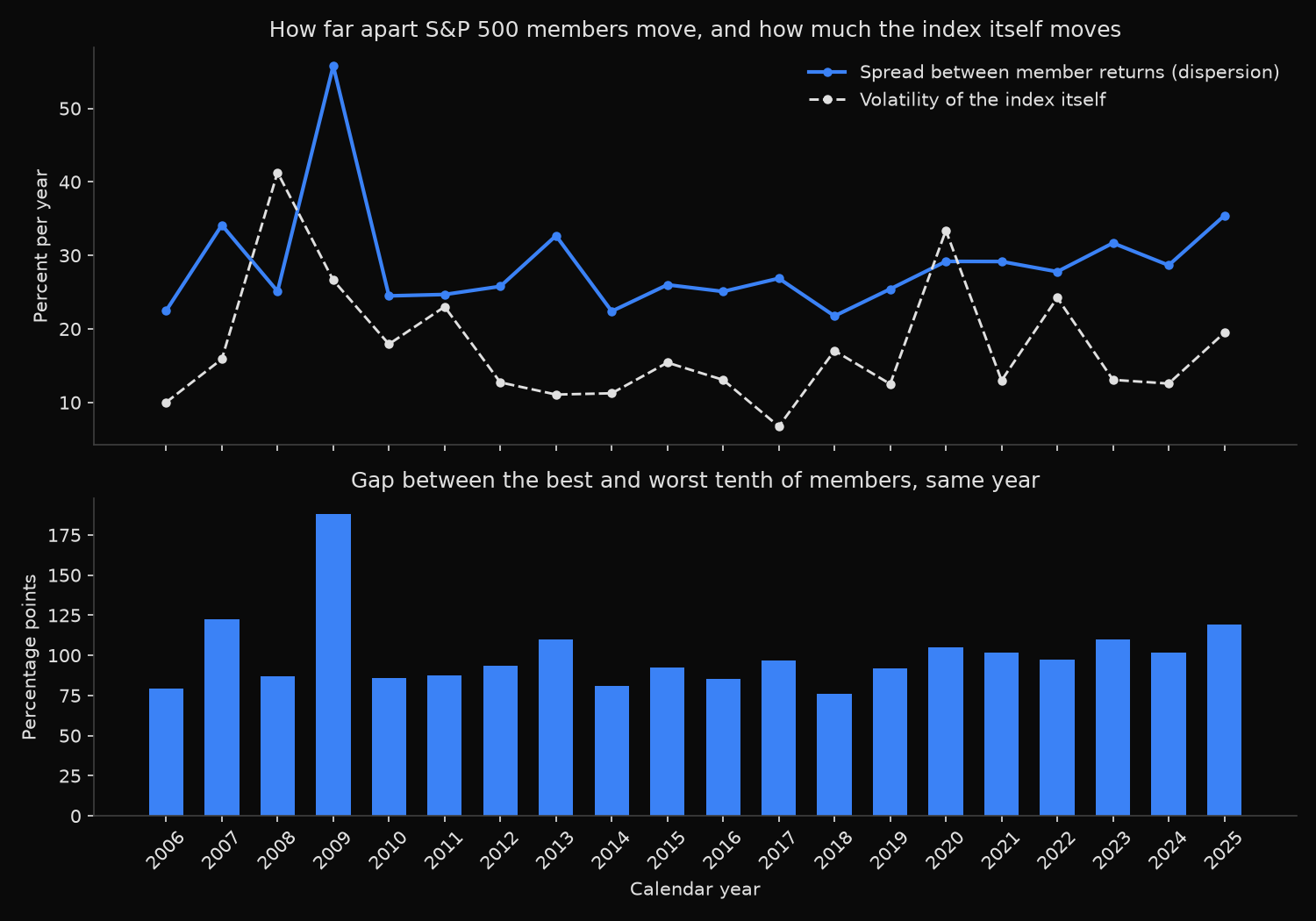
S&P 500 cross-sectional return dispersion, 2006-2025
point-in-time membership, 9,532 member-years, 250-253 trading days per year

year  members  dispersion  index vol  index return   top decile  bottom decile  decile spread
---------------------------------------------------------------------------------------------
2006      447       22.5%      10.0%       +15.8%       +57.1%        -22.0%         79.1pp
2007      443       34.1%      15.9%        +5.1%       +70.1%        -52.4%        122.5pp
2008      457       25.1%      41.3%       -36.8%        +5.1%        -82.0%         87.1pp
2009      464       55.8%      26.6%       +26.4%      +171.2%        -17.0%        188.2pp
2010      466       24.5%      17.9%       +15.1%       +68.7%        -17.1%         85.8pp
2011      469       24.7%      23.0%        +1.9%       +43.5%        -44.0%         87.5pp
2012      474       25.8%      12.7%       +16.0%       +68.9%        -24.8%         93.6pp
2013      479       32.7%      11.1%       +32.3%      +101.1%         -8.5%        109.7pp
2014      485       22.4%      11.2%       +13.5%       +53.2%        -27.6%         80.7pp
2015      474       26.0%      15.4%        +1.3%       +43.5%        -48.7%         92.2pp
2016      475       25.1%      13.1%       +12.0%       +59.7%        -25.7%         85.4pp
2017      484       26.9%       6.7%       +21.7%       +68.5%        -28.4%         97.0pp
2018      478       21.8%      17.0%        -4.6%       +32.3%        -43.8%         76.1pp
2019      486       25.4%      12.5%       +31.2%       +75.0%        -17.0%         92.0pp
2020      490       29.2%      33.4%       +18.4%       +68.6%        -36.5%        105.1pp
2021      493       29.2%      13.0%       +28.7%       +86.9%        -14.7%        101.6pp
2022      490       27.8%      24.2%       -18.2%       +45.0%        -52.4%         97.4pp
2023      495       31.7%      13.1%       +26.2%       +80.7%        -29.3%        110.0pp
2024      494       28.7%      12.6%       +24.9%       +68.8%        -33.0%        101.8pp
2025      489       35.4%      19.5%       +16.4%       +83.4%        -35.9%        119.3pp

widest dispersion    2009  55.8%   (index volatility 26.6%)
narrowest dispersion 2018  21.8%   (index volatility 17.0%)
loudest index        2008  index volatility 41.3%, dispersion 25.1%

average dispersion 28.7%, median 26.4%

dispersion against index volatility, same year   r=+0.22  p=0.351  rank r=+0.19
dispersion against index volatility, prior year  r=+0.58  p=0.009  rank r=+0.08
   leaving one year out, that r runs +0.02 to +0.64; without 2009 alone it is +0.02
dispersion against its own prior year            r=-0.20  p=0.400

decile spread divided by dispersion: mean 3.51, range 3.35-3.63  (3.51 if annual returns were normal)
What this tells us
Dispersion is never small. The narrowest year of the twenty, 2018, still put a standard deviation of 21.8 percent across the members, and the average year sits at 28.7 percent.
The comparison with index volatility is where the two ideas separate. Their correlation across the 20 years is +0.22 with a p-value of 0.35, and the rank correlation is +0.19; neither is distinguishable from zero. Two consecutive years show why. 2008 was the most violent year for the index in the sample at 41.3 percent volatility, yet its members finished 25.1 percent apart, below the 20-year average, because nearly everything fell at once. 2009 was calmer for the index at 26.6 percent volatility and produced the widest cross-section here, 55.8 percent, because the recovery was wildly uneven: the best tenth of members gained 171 percent while the worst tenth still lost 17 percent.
The lagged test looks more promising at first reading and then falls apart. Dispersion against the prior year’s index volatility gives r = +0.58 with p = 0.009, which would pass a casual significance check. The rank correlation on those pairs is +0.08, and refitting 19 times while holding out one year each time sends it as low as +0.02, which is what dropping 2009 alone produces. One pair of observations carries the result. Dispersion does not forecast its own next value either, at r = −0.20.
One relationship in the table is stable. The decile spread divided by dispersion averages 3.51 and stays between 3.35 and 3.63 in every year, and a normal distribution produces exactly 3.51. The gap between the best and worst tenth therefore carries no information beyond the standard deviation itself, which holds in 2009 with a member up 420 percent in it and in 2018 with nothing above 80 percent.
So what?
Dispersion converts directly into the size of a selection decision. Multiply the year’s dispersion by 3.5 and the result is the expected gap between a top-decile pick and a bottom-decile pick: 76 points in 2018, 188 points in 2009, 119 points in 2025. Any active risk budget or position limit is set against that number whether or not it has been measured.
Volatility is not a usable proxy for it. A calm index does not mean the members move together, which 2017 shows cleanly: the quietest index in the sample at 6.7 percent volatility, with a middling 26.9 percent dispersion beneath it. Waiting for a volatility spike before taking concentrated positions means waiting on an unrelated signal.
Since nothing tested here forecasts dispersion, it has to be measured as it happens. The same calculation runs on a rolling 60-day window of daily returns instead of a calendar year, giving a live reading of what the cross-section currently pays for being right. Without it, a 5-point win in 2018 and a 5-point win in 2009 look like the same achievement.
Built with xfinlink — free financial data API for Python.