How Much Does a Stock Fall on Its Ex-Dividend Date? Event Study in Python

August 31, 2026

What’s the question?

The ex-dividend date is the first morning on which a buyer of the share no longer receives the dividend the company has declared. Hold it at the previous close and the cash arrives; buy at the open and it does not. Value of a known size leaves the share overnight, so the price should open lower by exactly that amount, or a trader could buy at yesterday’s close, collect the dividend, sell into today’s open and pocket the difference.

That argument has been failing its own test since 1970, when Elton and Gruber measured the drop-to-dividend ratio and found it significantly below one. Differential taxation explains part of the gap: a taxable holder is indifferent at a drop worth less than the gross dividend, so the ratio reports the marginal holder’s valuation rather than an accounting identity. Trading costs explain more of it, since a discrepancy smaller than a round trip through the spread is one nobody removes. How far below one it sits has to be measured.

The approach

The sample is every ex-dividend event for the 497 S&P 500 members recorded on 31 December 2025, across 2021 through 2025. A positive dividend on a row of the daily price series marks an ex-dividend date, which the total-return column confirms: on those dates, and only those, the reported daily return equals the price change plus the dividend.

1. Take the raw drop as the previous session’s close minus the ex-date open. The open is the first price at which the share trades without the dividend attached, so it holds the event and little else.
2. Divide that drop by the dividend. Theory places the result at 1.0.
3. Remove the market: estimate each name’s beta against SPY on five years of daily returns, then subtract beta times the market’s own overnight move before forming the ratio.
4. Repeat using the ex-date close, and split the events into quartiles by dividend size relative to price, where the tax explanation makes a second prediction.

Four screens run first: both prices present with no gap in the series, no split on the ex-date or the session before it, a dividend no larger than 2 percent of the previous close, and an overnight move inside 10 percent. The dividend screen carries the weight, since specials and spin-offs are recorded exactly like quarterly payments and one 90-dollar special would rewrite a mean of ordinary ones. The screens remove 83 events of 7,773, 66 of them for dividend size.

Code

import numpy as np
import pandas as pd
import xfinlink as xfl

xfl.set_api_key("YOUR_API_KEY")  # free at https://xfinlink.com/signup

START, END = "2021-01-01", "2025-12-31"

spy = xfl.prices("SPY", start=START, end=END,
                 fields=["open", "close", "return_daily"]).sort_values("date")
spy["mkt_overnight"] = spy["open"] / spy["close"].shift(1) - 1.0
spy = spy[["date", "return_daily", "mkt_overnight"]].rename(
    columns={"return_daily": "mkt_total"})

ids = sorted({int(e) for e in xfl.index("sp500", as_of=END)["entity_id"].dropna()})
px = pd.concat([xfl.prices(entity_id=ids[i:i + 10], start=START, end=END,
                           fields=["open", "close", "dividend", "return_daily",
                                   "split_ratio"], max_rows=200_000)
                for i in range(0, len(ids), 10)], ignore_index=True)
px = (px.drop_duplicates(["entity_id", "date"]).sort_values(["entity_id", "date"])
        .reset_index(drop=True).merge(spy, on="date", how="left"))

grp = px.groupby("entity_id", sort=False)
px["prev_close"] = grp["close"].shift(1)
px["prev_date"] = grp["date"].shift(1)
px["prev_split"] = grp["split_ratio"].shift(1)

fit = px.dropna(subset=["return_daily", "mkt_total"])
fit = fit[fit["return_daily"].abs() <= 0.25]
beta = (fit.groupby("entity_id")
           .apply(lambda d: np.cov(d["return_daily"], d["mkt_total"])[0, 1]
                  / np.var(d["mkt_total"], ddof=1), include_groups=False).rename("beta"))

ev = px[px["dividend"] > 0].dropna(subset=["prev_close", "open", "mkt_overnight"])
ev = ev[(ev["date"] - ev["prev_date"]).dt.days <= 5]
ev = ev[ev["split_ratio"].isna() & ev["prev_split"].isna()].copy()
ev["div_yield"] = ev["dividend"] / ev["prev_close"]
ev = ev[ev["div_yield"] <= 0.02]
ev = ev[(ev["open"] / ev["prev_close"] - 1.0).abs() <= 0.10]
ev = ev.join(beta, on="entity_id").dropna(subset=["beta"])

ev["raw"] = (ev["prev_close"] - ev["open"]) / ev["dividend"]
ev["adj"] = (ev["prev_close"] - ev["open"]
             + ev["beta"] * ev["mkt_overnight"] * ev["prev_close"]) / ev["dividend"]

print(len(ev), ev["raw"].median(), ev["adj"].mean(), ev["adj"].median())
print(ev.groupby(pd.qcut(ev["div_yield"], 4))["adj"].agg(["size", "mean", "median"]))

Full script with formatting and visualisation: ex-dividend-day-price-drop-python.py

Output

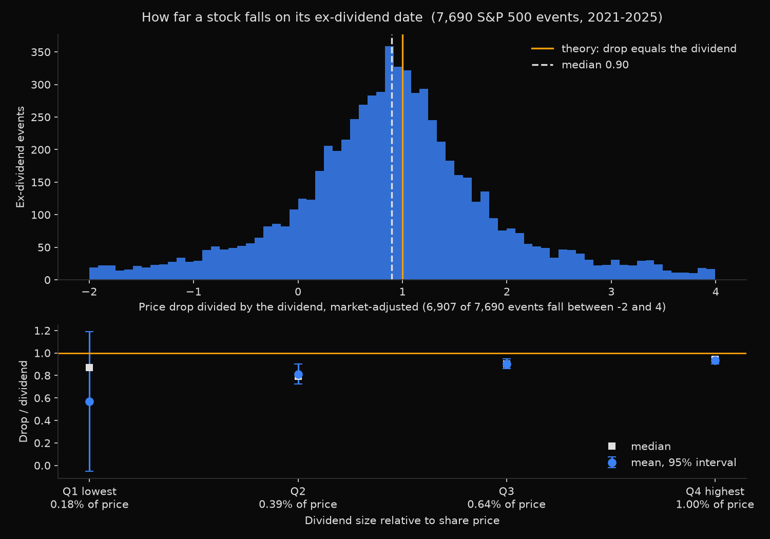
S&P 500 ex-dividend events, 2021-01-01 to 2025-12-31
members 497  payers 406  raw events 7773  kept 7690

  dropped    11  incomplete price pair
  dropped     0  gap in the price series
  dropped     2  split on or beside the ex-date
  dropped    66  dividend above 2% of price
  dropped     4  overnight move beyond the artefact ceiling

                        N     mean      SE   median      IQR   <1.0    <0
raw, open               7690    0.546   0.148    0.827   0.00-1.58  56.6% 24.7%
market-adjusted, open   7690    0.804   0.080    0.899   0.28-1.49  55.4% 18.8%
market-adjusted, close  7690    0.832   0.206    0.945  -0.60-2.47  51.3% 33.0%

pooled drop / pooled dividend  0.880    slope of drop on dividend, through the origin  0.935

market-adjusted ratio by dividend size (quartiles of dividend / price)
bucket          N   median yield     mean      SE   median
Q1 lowest     1923        0.18%    0.568   0.316    0.870
Q2            1922        0.39%    0.812   0.045    0.793
Q3            1922        0.64%    0.904   0.022    0.901
Q4 highest    1923        1.00%    0.933   0.015    0.942

shortfall per event: 6.2 bps of the share price, per-event sd 69 bps, t = 7.9

market-adjusted median by year
  2021: 0.879 (N=1475)  2022: 0.882 (N=1514)  2023: 0.896 (N=1540)  2024: 0.905 (N=1563)  2025: 0.922 (N=1598)

What this tells us

Every estimator lands below one and none near zero: median 0.899, mean 0.804 with a standard error of 0.080, pooled drop over pooled dividend 0.880, and a slope through the origin of 0.935. A dollar of dividend takes 88 to 94 cents of share price with it, depending on how much weight the estimator gives the largest payments.

Removing the market changes the headline: unadjusted, the mean falls to 0.546 and the median to 0.827, because the market drifted upward overnight across these five years and carried the ex-date open with it. Open against close matters more. The two centre in similar places, 0.899 and 0.945, but the interquartile range widens from 0.28-1.49 to -0.60-2.47 and the standard error nearly triples.

Precision is the part worth reading slowly. In the lowest quartile of dividend size, where the median payment is 0.18 percent of the share price, the mean comes out at 0.568 with a standard error of 0.316, which says nothing. In the highest quartile, at 1.00 percent, it is 0.933 with a standard error of 0.015, sitting 4.5 standard errors below one. Across the three quartiles carrying usable precision the ratio climbs with dividend size: 0.812, 0.904 and 0.933 in the means, 0.793, 0.901 and 0.942 in the medians. That is the second half of Elton and Gruber’s finding, reproduced 55 years later. Yearly medians rise every year, 0.879 to 0.922, which five observations cannot call a trend.

So what?

The gap is worth 6.2 basis points of the share price per event, against a standard deviation across events of 69 basis points. That is the whole prize in a dividend-capture trade, gross of everything. A round trip in a large cap crosses the spread twice and carries a night of market exposure a beta hedge only partly removes, so edge and friction come out the same size, which is what the transaction-cost explanation predicts.

Measuring the ratio on another universe turns on three settings: use the open, subtract the market, and screen out anything paying above about 2 percent of price on a single date. Names paying under roughly 0.3 percent per quarter produce nothing interpretable at all.

At 0.933 in the highest-dividend quartile, the marginal holder treats a dollar of dividend as worth about 93 cents of capital gain. Anyone modelling after-tax returns or setting payout policy is already using a number of that kind, and here it sits closer to one than the older literature would suggest.

Built with xfinlink — free financial data API for Python. pip install -U xfinlink