
What’s the question?
Mean-variance optimization needs an expected return for every asset it holds, and nobody has one.
Reverse optimization avoids the forecast. The argument goes back to William Sharpe in 1974 and now anchors the Black-Litterman model: assume the capitalisation-weighted index is already the optimal portfolio for a representative investor, then solve for the excess return vector that makes it optimal. That vector is mu = lambda * Sigma * w, with w the market weights, Sigma the covariance matrix of returns, and lambda a single risk-aversion number.
The output is known as equilibrium returns and serves as Black-Litterman’s neutral prior. What is inside that prior, and has it been right?
The approach
Nine formation dates, one at each year end from 2016 to 2024, each with the following twelve months held out. Members are addressed by entity id rather than ticker: a symbol on a 2016 roster can belong to an unrelated company in 2026.
- Pull the point-in-time roster at each year end, then weekly total returns, closing prices and share counts for the union of the nine rosters, 2014 through 2025.
- At each formation date, form weights from each member’s market value and estimate the annualised covariance matrix from the preceding three years of weekly returns.
- Set lambda so the index prices a 5 percent annual risk premium, then compute mu = lambda * Sigma * w. That choice scales the vector and leaves its ordering untouched.
- Measure the next twelve months for each member: total return, return above one-to-three month Treasury bills, annualised weekly volatility, worst drawdown.
- Sort into quintiles by implied return, equal weight within each, and average across the nine cross-sections.
Weekly returns pass a consistency screen against the price path first, since an equal-weighted average is sensitive to one extreme value; four of 373,948 observations fail it. Members without a complete three-year series and a full forward year drop from that cross-section, leaving 482 of roughly 500. The reconstructed capitalisation-weighted series correlates 0.988 to 0.998 weekly with SPY.
Code
import numpy as np
import pandas as pd
import xfinlink as xfl

xfl.set_api_key("YOUR_API_KEY")  # free at https://xfinlink.com/signup

ERP = 0.05
roster = xfl.index("sp500", as_of="2024-12-31")
ids = [int(i) for i in roster["entity_id"]]

px = pd.concat([xfl.prices(entity_id=ids[i:i + 25], start="2022-01-01", end="2024-12-31",
                           interval="1w", fields=["date", "return_daily", "close",
                                                  "shares_outstanding"])
                for i in range(0, len(ids), 25)], ignore_index=True)

ret = px.pivot_table(index="date", columns="entity_id", values="return_daily").dropna(axis=1)
mcap = (px.pivot_table(index="date", columns="entity_id", values="close")
        * px.pivot_table(index="date", columns="entity_id", values="shares_outstanding"))

cap = mcap[ret.columns].ffill().iloc[-1]
w = (cap / cap.sum()).to_numpy()
R = ret.to_numpy()

cov = np.cov(R, rowvar=False) * 52.0
implied = (ERP / (w @ cov @ w)) * (cov @ w)          # mu = lambda * Sigma * w

rp = R @ w                                           # the index's own return series
beta = np.array([np.cov(R[:, j], rp)[0, 1] / np.var(rp, ddof=1)
                 for j in range(R.shape[1])])

print(f"implied return range: {implied.min():.2%} to {implied.max():.2%}")
print(f"max |mu - ERP x beta|: {np.max(np.abs(implied - ERP * beta)):.1e}")
Full script: reverse-optimization-implied-returns-python.py
Output
------------------------------------------------------------------------------
REVERSE OPTIMIZATION OF THE S&P 500, FORMATION YEAR ENDS 2016-2024
implied excess return mu = lambda * Sigma * w, lambda set so the index
prices a 5% annual risk premium
------------------------------------------------------------------------------
universe: point-in-time S&P 500 members at each year end, addressed by
          entity id; 3 years of weekly returns behind each formation
          date and 12 months in front of it, 482 members per year on average
weekly observations 373,948; set aside by the consistency screen: 4

PER FORMATION
year   names  index vol  lambda  implied lo  implied hi  max |mu-ERPb|  corr w/ SPY
2017     477      12.5%    3.20      -0.20%      13.11%        1.2e-16        0.998
2018     476      11.5%    3.81       0.16%      14.17%        1.2e-16        0.997
2019     482      13.3%    2.84      -0.11%      12.06%        5.6e-17        0.997
2020     487      12.7%    3.09       0.48%      10.09%        1.1e-16        0.997
2021     483      22.5%    0.99       0.84%      12.08%        9.7e-17        0.995
2022     480      21.3%    1.10      -0.80%      13.47%        1.4e-16        0.995
2023     487      23.9%    0.87       0.88%      12.65%        1.2e-16        0.996
2024     491      17.8%    1.57       0.43%      10.60%        9.7e-17        0.996
2025     481      19.2%    1.36       0.06%      10.52%        8.3e-17        0.988

IMPLIED-RETURN QUINTILES, AVERAGE OF THE NINE CROSS-SECTIONS
quintile        n  implied   beta  excess ret   median  volatility  drawdown  ret/vol
Q1 lowest      97    2.54%   0.51       5.94%    5.77%       25.2%    -19.8%     0.24
Q2             96    4.08%   0.82       8.38%    7.86%       27.9%    -22.1%     0.30
Q3             96    4.99%   1.00       9.69%    8.41%       30.0%    -24.2%     0.32
Q4             96    5.83%   1.17      10.18%    8.14%       31.4%    -25.7%     0.32
Q5 highest     97    7.63%   1.53      12.12%    7.13%       37.8%    -30.6%     0.32

growth of $1 held in each quintile, equal weighted, rebalanced every year:
  Q1 1.98x  Q2 2.38x  Q3 2.62x  Q4 2.69x  Q5 3.09x

RANK CORRELATION OF THE IMPLIED RETURN WITH WHAT FOLLOWED
year    vs 12m return   vs 12m volatility   index return
2017           +0.150              +0.396          21.3%
2018           -0.288              +0.501          -3.2%
2019           -0.029              +0.544          30.4%
2020           +0.161              +0.230          20.7%
2021           +0.178              +0.543          28.5%
2022           -0.117              +0.417         -18.6%
2023           +0.203              +0.478          23.9%
2024           -0.003              +0.530          25.2%
2025           +0.017              +0.551          16.0%
mean           +0.030              +0.466          16.0%

FORMED 31 DEC 2024: THE ENDS OF THE IMPLIED-RETURN RANKING
ticker  company                           beta  implied  2025 return
GIS     General Mills Inc                 0.01    0.06%       -27.2%
CPB     Campbells Co                      0.05    0.27%       -33.2%
KHC     Kraft Heinz Co                    0.12    0.61%       -20.8%
SJM     Smucker J M Co                    0.12    0.62%       -12.3%
NVDA    Nvidia Corp                       2.10   10.52%        29.1%
PLTR    Palantir Technologies Inc         2.07   10.35%       122.5%
TSLA    Tesla Inc                         1.91    9.53%         9.6%
CZR     Caesars Entertainment Inc De      1.89    9.43%       -28.1%
What this tells us
The i-th element of Sigma * w is the covariance between member i and the market portfolio, and beta is that same covariance divided by the market’s variance, so mu_i collapses to the assumed risk premium multiplied by beta_i. The column headed max |mu-ERPb| measures the gap and never exceeds 1.4e-16, floating-point noise rather than a difference. A covariance matrix holding some 115,000 distinct entries yields one number per member, and that number is beta. Beta multiplied by a risk premium is also the textbook route to a discount rate, which a CAPM cost-of-equity estimate walks through.
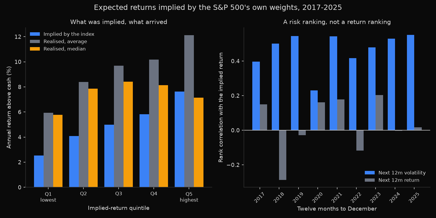
As a forecast the vector splits cleanly in two. Its ranking of risk holds every year: the rank correlation with realised volatility runs from +0.230 to +0.551, positive in all nine years, averaging +0.466, and the drawdown ordering agrees, at 19.8 percent from peak for the lowest quintile against 30.6 percent for the highest. Its ranking of return holds in no particular year: -0.288 in 2018, +0.203 in 2023, negative in four of nine years, averaging +0.030.
Averaged over the nine cross-sections, though, the levels line up: implied returns rise from 2.54 to 7.63 percent across the quintiles, realised excess returns from 5.94 to 12.12 percent, and a dollar in the lowest quintile grew to $1.98 against $3.09 in the highest. Beta was compensated, roughly in the proportion assumed.
The medians complicate that. They peak in the middle rather than at the top, so the typical member of the highest-implied quintile did worse than the typical member of the third, and the gap between Q5’s 12.12 percent mean and its 7.13 percent median is a right tail doing the work, Palantir’s 122.5 percent in 2025 among them. Return per unit of realised volatility settles at 0.32 across the top three quintiles against 0.24 at the bottom.
So what?
Anyone running Black-Litterman starts from a beta ranking. The prior holds no view on quality, valuation or growth; it says riskier names should return more, in exact proportion. A view is worth expressing only where it carries information beta does not already contain.
Where the vector earns its place is as a risk statement that costs no forward-looking estimate. Use it to set risk budgets and to price how much extra volatility a tilt buys.
Do not use it to pick stocks for the coming year. General Mills entered 2025 carrying an implied excess return of 0.06 percent on a beta of 0.01, then fell 27.2 percent. An equilibrium model prices systematic risk and says nothing about the risk that a company’s own business deteriorates.
Built with xfinlink — free financial data API for Python.