
How Often Does a 99% Value-at-Risk Limit Actually Break? VaR Backtesting in Python
August 3, 2026
What’s the question?
Value at risk compresses a portfolio’s downside into one number. A 99 percent one-day VaR of 3 percent says a loss worse than 3 percent belongs to the worst day in a hundred. Basel grades a bank’s internal model by counting how many of the previous 250 days broke through.
A correct 99 percent model breaks on one percent of days. That is the easy half. The harder half is when the breaks arrive: a model that delivers every one of its failures inside three weeks is useless at the moment capital is at stake.
Two likelihood ratio tests separate the halves. The unconditional coverage test of Kupiec (1995) compares the observed breach frequency against the promised one percent. The independence test of Christoffersen (1998) fits a two-state Markov chain to the breach sequence and asks whether a breach today changes the probability of a breach tomorrow; under a correct model it does not. A model can pass the first test and fail the second.
The approach
Eight exchange-traded funds cover US large cap (SPY), US small cap (IWM), developed markets outside the US (EFA), emerging markets (EEM), long Treasuries (TLT), investment grade credit (LQD), high yield credit (HYG), and listed real estate (VNQ). Returns are daily price changes on the split-adjusted close.
- Each session, estimate the one-day 99 percent VaR from the 500 sessions ending at the previous close. The Gaussian model uses the window mean plus its standard deviation times the normal first percentile; historical simulation uses the window’s own first percentile, assuming nothing about shape.
- Record a breach whenever the realised return falls below that morning’s number. Evaluation runs 4 January 2016 to 31 July 2026: 2,659 sessions per fund, 26.6 breaches expected.
- Run Kupiec, Christoffersen, and the joint statistic, their sum against a chi-square with two degrees of freedom.
- Repeat everything on 60,000 simulated normal returns and on simulated breach sequences, as controls for estimation noise and test size.
Both statistics were checked against second implementations built from different formulas, and the rolling window against an explicit loop and a look-ahead probe.
Code
import numpy as np
import pandas as pd
import xfinlink as xfl
from scipy import stats

xfl.set_api_key("YOUR_API_KEY")  # free at https://xfinlink.com/signup

ASSETS = ["SPY", "IWM", "EFA", "EEM", "TLT", "LQD", "HYG", "VNQ"]
WINDOW, ALPHA = 500, 0.01

px = xfl.prices(ASSETS, start="2013-06-01", end="2026-07-31", fields=["adj_close"])


def _xlogy(a, b):
    return 0.0 if a == 0 else a * np.log(b)


def kupiec(hits, p):
    """Unconditional coverage: is the breach rate p? LR ~ chi2(1)."""
    n, x = len(hits), int(hits.sum())
    pi = x / n
    lr = 2 * ((_xlogy(n - x, 1 - pi) + _xlogy(x, pi))
              - (_xlogy(n - x, 1 - p) + _xlogy(x, p)))
    return lr, 1 - stats.chi2.cdf(lr, 1)


def christoffersen(hits):
    """Independence: does a breach today change the odds of one tomorrow?"""
    a, b = hits[:-1], hits[1:]
    n00 = int(((a == 0) & (b == 0)).sum()); n01 = int(((a == 0) & (b == 1)).sum())
    n10 = int(((a == 1) & (b == 0)).sum()); n11 = int(((a == 1) & (b == 1)).sum())
    pi = (n01 + n11) / (n00 + n01 + n10 + n11)
    p01 = n01 / (n00 + n01) if n00 + n01 else 0.0
    p11 = n11 / (n10 + n11) if n10 + n11 else 0.0
    lr = 2 * ((_xlogy(n00, 1 - p01) + _xlogy(n01, p01)
               + _xlogy(n10, 1 - p11) + _xlogy(n11, p11))
              - (_xlogy(n00 + n10, 1 - pi) + _xlogy(n01 + n11, pi)))
    return lr, 1 - stats.chi2.cdf(lr, 1)


for t in ASSETS:
    s = px[px["ticker"] == t].sort_values("date").reset_index(drop=True)
    s["ret"] = s["adj_close"].pct_change()
    s = s.dropna(subset=["ret"]).reset_index(drop=True)

    roll = s["ret"].shift(1).rolling(WINDOW)          # window ends yesterday
    s["gauss"] = roll.mean() + roll.std(ddof=1) * stats.norm.ppf(ALPHA)
    s["hist"] = roll.quantile(ALPHA)

    ev = s[(s["date"] >= "2016-01-01") & s["gauss"].notna()]
    for col in ("gauss", "hist"):
        h = (ev["ret"] < ev[col]).to_numpy().astype(int)
        print(f"{t} {col}: {h.sum()} breaches, rate {h.mean():.2%}, "
              f"Kupiec p={kupiec(h, ALPHA)[1]:.4f}, "
              f"independence p={christoffersen(h)[1]:.4f}")
Full script with formatting and visualisation: value-at-risk-backtest-kupiec-christoffersen-python.py
Output
Series check
  SPY   3311 rows  2013-06-03 to 2026-07-31  worst day -10.94%  best day +10.50%  missing values 0
  IWM   3311 rows  2013-06-03 to 2026-07-31  worst day -13.27%  best day +9.15%  missing values 0
  EFA   3311 rows  2013-06-03 to 2026-07-31  worst day -10.99%  best day +8.47%  missing values 0
  EEM   3311 rows  2013-06-03 to 2026-07-31  worst day -12.48%  best day +8.05%  missing values 0
  TLT   3311 rows  2013-06-03 to 2026-07-31  worst day -6.67%  best day +7.52%  missing values 0
  LQD   3311 rows  2013-06-03 to 2026-07-31  worst day -5.00%  best day +7.39%  missing values 0
  HYG   3311 rows  2013-06-03 to 2026-07-31  worst day -5.50%  best day +6.55%  missing values 0
  VNQ   3311 rows  2013-06-03 to 2026-07-31  worst day -17.73%  best day +9.00%  missing values 0

One-day 99% value-at-risk backtest, daily price returns
Rolling 500-day estimation window, evaluated 2016-01-04 to 2026-07-31
2659 trading days per fund, 26.6 breaches expected if the model is right

Gaussian VaR  (window mean and standard deviation, normal quantile)
                         avg VaR  breaches    rate   Kupiec p   Indep p   Joint p
SPY  US large cap         -2.47%        69   2.59%    0.0000*   0.0000*   0.0000*
IWM  US small cap         -3.17%        51   1.92%    0.0000*   0.0000*   0.0000*
EFA  Developed ex-US      -2.48%        55   2.07%    0.0000*   0.0311*   0.0000*
EEM  Emerging markets     -2.97%        57   2.14%    0.0000*   0.0401*   0.0000*
TLT  20y+ Treasuries      -2.17%        32   1.20%    0.3069    0.0061*   0.0137*
LQD  Investment grade     -1.17%        44   1.65%    0.0019*   0.0000*   0.0000*
HYG  High yield           -1.19%        57   2.14%    0.0000*   0.0000*   0.0000*
VNQ  US REITs             -2.88%        52   1.96%    0.0000*   0.0004*   0.0000*
  mean breach rate 1.96%   funds failing Kupiec at 5%: 7/8   failing independence: 8/8

Historical VaR  (1st percentile of the window)
                         avg VaR  breaches    rate   Kupiec p   Indep p   Joint p
SPY  US large cap         -3.10%        42   1.58%    0.0056*   0.0000*   0.0000*
IWM  US small cap         -3.83%        37   1.39%    0.0554    0.0001*   0.0001*
EFA  Developed ex-US      -3.06%        39   1.47%    0.0237*   0.0201*   0.0052*
EEM  Emerging markets     -3.42%        41   1.54%    0.0093*   0.0270*   0.0029*
TLT  20y+ Treasuries      -2.10%        34   1.28%    0.1662    0.0088*   0.0124*
LQD  Investment grade     -1.34%        30   1.13%    0.5149    0.0000*   0.0000*
HYG  High yield           -1.42%        34   1.28%    0.1662    0.0000*   0.0000*
VNQ  US REITs             -3.50%        33   1.24%    0.2286    0.0684    0.0921
  mean breach rate 1.36%   funds failing Kupiec at 5%: 3/8   failing independence: 7/8

Breach timing, historical simulation VaR (2020-02-20 to 2020-04-30 is 50 of the 2659 sessions, 1.9%)
  SPY    42 breaches   10 in the crisis window (23.8%)    21 within a week of the previous one (50.0%)
  IWM    37 breaches    9 in the crisis window (24.3%)    13 within a week of the previous one (35.1%)
  EFA    39 breaches    9 in the crisis window (23.1%)    12 within a week of the previous one (30.8%)
  EEM    41 breaches    7 in the crisis window (17.1%)    10 within a week of the previous one (24.4%)
  TLT    34 breaches    5 in the crisis window (14.7%)    10 within a week of the previous one (29.4%)
  LQD    30 breaches    8 in the crisis window (26.7%)    12 within a week of the previous one (40.0%)
  HYG    34 breaches   12 in the crisis window (35.3%)    17 within a week of the previous one (50.0%)
  VNQ    33 breaches    8 in the crisis window (24.2%)     9 within a week of the previous one (27.3%)
  all funds: 290 breaches, 68 (23.4%) inside that window
  days on which all 8 funds breached at once: 2020-03-11, 2020-03-18, 2022-06-13

Calibration on data with no fat tails and no volatility clustering
  60,000 simulated independent normal returns: Gaussian VaR breached 1.02% of days, historical simulation 1.19%
  simulated 2659-day breach sequences, tests run at the 5% level:
    genuinely independent 1% breaches: Kupiec rejects 6.3%, independence rejects 1.5%
    clustered breaches, same 1% rate  : Kupiec rejects 17.2%, independence rejects 99.8%
What this tells us
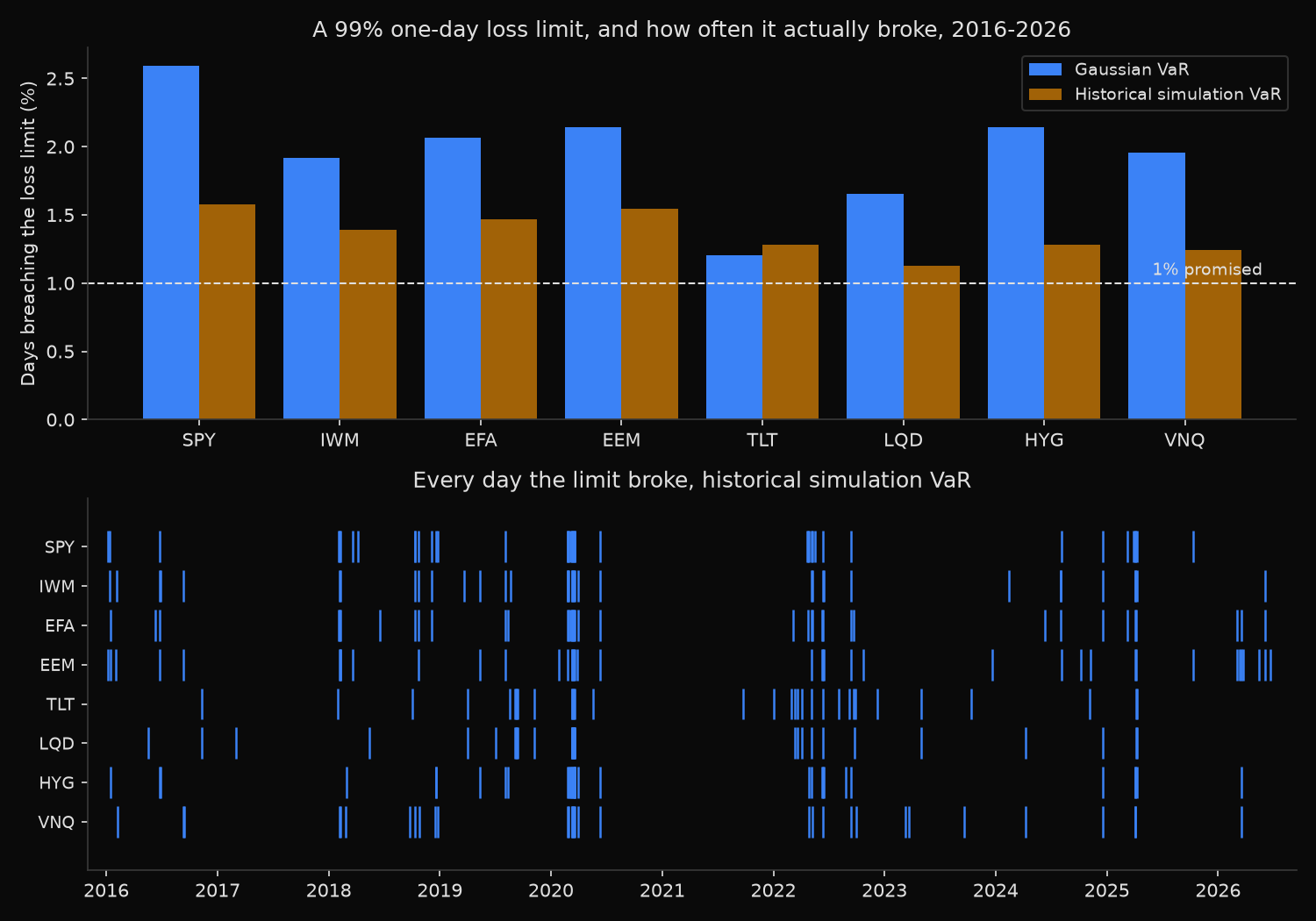
The Gaussian model broke on 1.96 percent of days averaged across the eight funds, close to double its promise, and seven reject Kupiec’s test. SPY is worst at 2.59 percent: 69 breaches against 27 expected. TLT alone survives on count.
Historical simulation cuts most of that excess, to 1.36 percent, with three funds rejecting. Part of the remainder is not fat tails: the same estimator on 60,000 simulated normal returns breached 1.19 percent, because the first percentile of 500 observations is itself noisy. Against that benchmark, historical simulation misses by little.
Timing is where both models come apart. Every fund rejects independence under the Gaussian model, and seven of eight still reject under historical simulation, VNQ the lone survivor at p = 0.068. Of the 290 historical-simulation breaches, 68 fell inside the 50 sessions between 20 February and 30 April 2020: 1.9 percent of the sample carried 23.4 percent of the failures, twelve times an even spread. All eight funds breached together on 11 March 2020, on 18 March 2020, and on 13 June 2022.
The mechanism is arithmetic: a 500-session window is two years long, so the limit standing on 12 March 2020 still averaged over 2018 and 2019. SPY’s worst session, a loss of 10.94 percent, ran more than three times past the limit set that morning.
The tests are not manufacturing these rejections. On simulated independent sequences the independence test fired only 1.5 percent of the time at a nominal 5 percent level, so it under-rejects here; on clustered sequences carrying exactly the right one percent rate it caught 99.8 percent against Kupiec’s 17.2 percent.
So what?
A breach count is not a validated model. Report the Christoffersen p-value beside it, for every asset, every quarter. The eight funds split cleanly: on count, five of the eight historical-simulation models look acceptable; on timing, seven are broken. A report carrying only the first column would have signed off on HYG, which passed on count and then broke twelve times in the ten weeks after 20 February 2020.
Historical simulation is the better of the two and costs one line of code. The fix for the clustering is a faster variance, not a different quantile: divide each window return by a volatility estimate that reacts within days, take the percentile of those residuals, then rescale by today’s volatility.
A 99 percent limit validated on frequency alone understates how much can go wrong in a fortnight. Size the buffer against the worst cluster in the backtest, not the average year.
Built with xfinlink — free financial data API for Python. pip install -U xfinlink
pip install -U xfinlink