
Do Sector Correlations Spike When the Market Falls? Conditional Beta Analysis in Python
September 13, 2026
What’s the question?
Diversification is supposed to fail at the moment it is needed. The usual phrasing is that correlations go to one in a crash, so a portfolio spread across sectors collapses into a single position on the day that matters. It is repeated often enough to work as an assumption rather than as a measurement.
Two quantities hide inside that sentence. Beta is the slope of a sector’s return against the market’s: a beta of 1.4 means the sector falls about 1.4% on a day the market falls 1%. Correlation measures how tightly the daily observations sit around that slope. Losses come from the slope; correlation only says how reliably the slope shows up.
The distinction becomes sharp once the sample is selected by market outcome. A slope estimated only on days the market fell hard is the same slope, provided the relationship is linear. A correlation is not, because it also depends on how widely the market itself moved inside the sample. Narrow the range of market outcomes and correlation drops, with nothing underneath having changed.
So the question divides in two: does sector correlation rise on the worst market days, and does the quantity that sets the size of the loss rise with it?
The approach
Nine sector funds against one market fund, across the dot-com decline, 2008, 2020 and 2022.
- Pull daily closes for SPY and the nine Select Sector SPDR funds from 1999 to the end of 2024. Each fund is one tradeable line with a continuous history, which holds the sector definition fixed across 26 years.
- Convert split-adjusted closes to daily returns, leaving 6,540 trading days shared by all ten series.
- Rank the days by market return and cut the worst decile, 654 days with SPY at or below -1.27%, plus the best decile for comparison.
- Regress each sector on the market three times: all days, worst decile, best decile. Record the slope, its standard error, and the correlation.
- Repeat the split with September to December 2008 and February to April 2020 deleted, so no single crisis carries the result.
Code
import numpy as np
import pandas as pd
import xfinlink as xfl

xfl.set_api_key("YOUR_API_KEY")  # free at https://xfinlink.com/signup

SECTORS = ["XLB", "XLE", "XLF", "XLI", "XLK", "XLP", "XLU", "XLV", "XLY"]

px = (pd.concat([xfl.prices(t, start="1999-01-01", end="2024-12-31",
                            fields=["adj_close"], max_rows=200000)
                 for t in ["SPY"] + SECTORS], ignore_index=True)
        .pivot(index="date", columns="ticker", values="adj_close")
        .sort_index())
ret = px.pct_change().dropna()

mkt = ret["SPY"]
worst = mkt <= mkt.quantile(0.10)        # 654 days, SPY at or below -1.27%
best = mkt >= mkt.quantile(0.90)


def fit(mask):
    out = {}
    for t in SECTORS:
        x, y = mkt[mask], ret[t][mask]
        b, a = np.polyfit(x, y, 1)                     # slope is beta
        resid = y - (a + b * x)
        se = resid.std(ddof=2) / (np.sqrt(len(x)) * x.std(ddof=0))
        out[t] = (b, se, np.corrcoef(x, y)[0, 1])
    return pd.DataFrame(out, index=["beta", "se", "corr"]).T


f_all = fit(pd.Series(True, index=mkt.index))
f_worst, f_best = fit(worst), fit(best)

print(f_all.join(f_worst, rsuffix="_worst").join(f_best, rsuffix="_best").round(3))
Full script with formatting and visualisation: sector-beta-market-crash-python.py
Output
==================================================================================
Sector beta and correlation on the worst 10% of market days
==================================================================================
Universe : SPY and the nine Select Sector SPDRs, daily price returns
Window   : 1999-01-05 to 2024-12-31   (6,540 trading days)
Buckets  : worst 10% = 654 days with SPY at or below -1.27%
           best 10%  = 654 days with SPY at or above +1.25%
Market return: mean -2.23% and standard deviation 1.13% inside the worst decile,
               against 1.22% across all days

Beta on the S&P 500 ETF
----------------------------------------------------------------------------------
Sector                          all days  worst 10%    s.e.  best 10%  worst - all
Energy (XLE)                       0.986      1.420   0.060     1.080       +0.434
Financials (XLF)                   1.233      1.477   0.053     1.331       +0.244
Utilities (XLU)                    0.620      0.813   0.044     0.799       +0.193
Materials (XLB)                    0.965      1.029   0.043     0.936       +0.064
Consumer Staples (XLP)             0.545      0.605   0.033     0.505       +0.060
Industrials (XLI)                  0.969      0.995   0.030     0.888       +0.027
Health Care (XLV)                  0.731      0.750   0.032     0.707       +0.019
Consumer Discretionary (XLY)       1.006      1.014   0.033     0.788       +0.008
Technology (XLK)                   1.159      0.887   0.037     1.088       -0.272
average                            0.913      0.999             0.902       +0.086

Correlation with the S&P 500 ETF
----------------------------------------------------------------------------------
Sector                          all days  worst 10%  best 10%  worst - all
Energy (XLE)                       0.661      0.678     0.565       +0.017
Financials (XLF)                   0.829      0.739     0.667       -0.091
Utilities (XLU)                    0.616      0.584     0.574       -0.032
Materials (XLB)                    0.784      0.680     0.659       -0.105
Consumer Staples (XLP)             0.689      0.577     0.504       -0.111
Industrials (XLI)                  0.883      0.796     0.775       -0.088
Health Care (XLV)                  0.790      0.671     0.686       -0.120
Consumer Discretionary (XLY)       0.859      0.770     0.660       -0.089
Technology (XLK)                   0.867      0.685     0.715       -0.182
average                            0.775      0.687     0.645       -0.089

Why correlation falls while beta rises
----------------------------------------------------------------------------------
Sector-specific volatility in the worst decile, relative to all days         1.35x
Correlation implied by holding beta and sector-specific volatility fixed     0.752
Correlation actually observed inside the worst decile                        0.687

Beta with September-December 2008 and February-April 2020 removed
----------------------------------------------------------------------------------
6,393 trading days, 640 of them in the worst decile
Sector                          all days  worst 10%  worst - all
Energy (XLE)                       0.880      1.082       +0.202
Financials (XLF)                   1.211      1.460       +0.250
Utilities (XLU)                    0.537      0.633       +0.096
Materials (XLB)                    0.953      1.009       +0.056
Consumer Staples (XLP)             0.533      0.551       +0.018
Industrials (XLI)                  0.986      1.117       +0.131
Health Care (XLV)                  0.739      0.852       +0.113
Consumer Discretionary (XLY)       1.040      1.035       -0.005
Technology (XLK)                   1.208      0.961       -0.246
==================================================================================
What this tells us
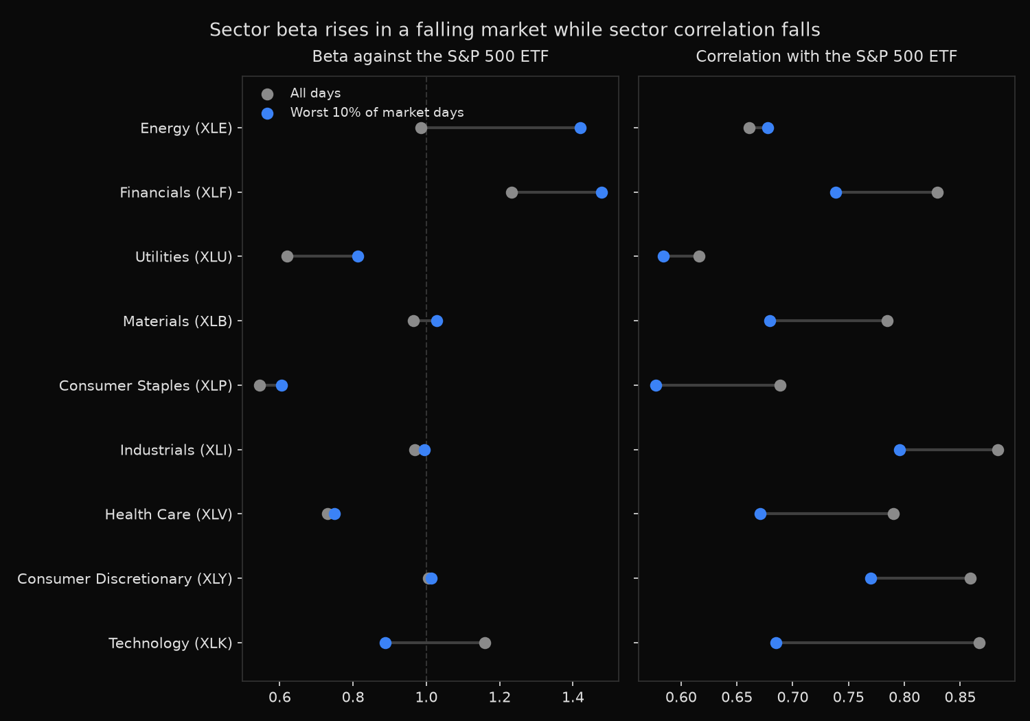
Correlation does not spike. It falls in eight of the nine sectors, from an average of 0.775 across all days to 0.687 inside the worst decile, with Health Care losing 0.120 and Technology 0.182. Only Energy rises, by 0.017.
Two forces produce that decline and the output separates them. The market’s own spread inside the worst decile is 1.13% against 1.22% across all days, while sector-specific movement grows to 1.35 times its normal size. Holding each sector’s beta and its sector-specific volatility fixed gives an expected 0.752, already below the full-sample 0.775. The observed 0.687 sits below that in turn, because idiosyncratic movement expands faster than market movement in a sell-off.
Beta answers differently. The average rises from 0.913 to 0.999, and the movement is concentrated: Energy 0.986 to 1.420, Financials 1.233 to 1.477, Utilities 0.620 to 0.813. Standard errors on the crash-day slopes run 0.030 to 0.060, so each of those shifts is several standard errors wide. Technology moves the other way, 1.159 to 0.887, and its best-decile beta of 1.088 is higher still, so much of technology’s full-sample beta is earned on rallies.
Deleting the two crisis stretches leaves the shape intact. Energy still gains 0.202, Financials 0.250, Technology still loses 0.246, and Health Care and Industrials gain more than they did in the full sample. The pattern belongs to falling markets generally, not to 2008 or March 2020.
So what?
Measure downside exposure with beta and leave conditional correlation out of it. A correlation computed inside a slice of market outcomes describes tightness within that slice, and it will usually come out below the full-sample figure it is compared against.
Re-estimate beta on the worst decile before sizing anything that has to survive a sell-off. A hedge sized on full-sample beta leaves 31% of Energy’s crash-day exposure uncovered and 17% of the exposure in Financials, while covering 131% of Technology’s. Utilities deserve attention: a beta of 0.620 describes a sector taking 38% less of a market decline than the market itself, and the figure that shows up on the days the market actually declines is 0.813.
The asymmetry runs both ways. Consumer Discretionary carries 1.014 into the worst days and 0.788 into the best, absorbing the fall and giving back less of the recovery; Technology carries 0.887 down and 1.088 up. Splitting one regression into two costs a single line of code and answers the question a full-sample beta averages away.
Built with xfinlink — free financial data API for Python. pip install -U xfinlink
pip install -U xfinlink