Do Corporate Insiders Time the Market? S&P 500 Insider Buying Breadth in Python

August 21, 2026

What’s the question?

Every officer, director and 10% owner of a listed US company must report trades in their own stock on Form 4, before the end of the second business day after the trade. Most work on that record examines one company at a time. Adding it up produces a monthly census of how many of the largest American companies had somebody on the inside putting personal money into the shares.

The claim attached to that census is a timing claim. Insiders are supposed to buy into falling prices and stay away when their own stock looks expensive, which would make aggregate purchase activity a read on the whole market rather than on any single name. Waves of buying get described as a floor and long stretches of silence as a warning, but neither half is usually tested against the index it is supposed to forecast.

Breadth here means the percentage of index constituents with at least one open-market purchase by an insider during a calendar month. Counting companies rather than dollars stops one large block trade from swamping the measure.

The approach

The sample is the S&P 500 on point-in-time membership, January 2010 to December 2025. What is being forecast is SPY, the fund that tracks the index, on a total-return basis.

1. Rebuild the roster as of 1 January of each year and key it on company identifier rather than ticker, since symbols get reassigned to different companies over time.
2. Pull every Form 4 open-market buy and sell for those companies. Grants, option exercises, tax withholding and gifts are excluded, because none of them is a decision about price.
3. Count the distinct companies with at least one purchase in each month, then divide by that year’s roster size.
4. Compound SPY daily total returns into calendar months and measure the return over the 3, 6 and 12 months after each month end.
5. Sort the months into quintiles by breadth and estimate the slope with Newey-West standard errors, lagged to the horizon, since overlapping forward windows would otherwise inflate every t-statistic.

The filing deadline matters for step 4. A month’s purchases are public by the time that month ends, apart from any placed in the final two sessions, so the month-end close is a fair entry point.

Code

import numpy as np
import pandas as pd
import statsmodels.api as sm
import xfinlink as xfl

xfl.set_api_key("YOUR_API_KEY")  # free at https://xfinlink.com/signup

frames, roster_size = [], {}
for year in range(2010, 2026):
    roster = xfl.index("sp500", as_of=f"{year}-01-01")
    ids = [int(e) for e in roster["entity_id"].dropna()]
    roster_size[year] = len(ids)
    for i in range(0, len(ids), 100):
        frames.append(xfl.insiders(
            entity_id=ids[i:i + 100], start=f"{year}-01-01", end=f"{year}-12-31",
            transaction_type=["open_market_buy", "open_market_sell"],
            fields=["entity_id", "transaction_date", "transaction_type"],
            max_rows=200_000))

trades = pd.concat(frames, ignore_index=True)
trades["transaction_date"] = pd.to_datetime(trades["transaction_date"]).dt.tz_localize(None)
trades["month"] = trades["transaction_date"].dt.to_period("M")

counts = (trades.groupby(["month", "transaction_type"])["entity_id"]
          .nunique().unstack(fill_value=0))
counts["buy_breadth"] = (100 * counts["open_market_buy"]
                         / [roster_size[m.year] for m in counts.index])

spy = xfl.prices("SPY", start="2009-12-01", end="2026-08-20",
                 fields=["close", "return_daily"])
spy["month"] = spy["date"].dt.to_period("M")
monthly = spy.groupby("month")["return_daily"].apply(lambda s: (1 + s).prod() - 1)

panel = counts.join(monthly.rename("spy_ret"), how="right").sort_index()
log_ret = np.log1p(panel["spy_ret"])
panel["fwd12"] = [np.expm1(log_ret.iloc[i + 1:i + 13].sum()) if i + 12 < len(panel)
                  else np.nan for i in range(len(panel))]

d = panel.dropna(subset=["buy_breadth", "fwd12"])
fit = sm.OLS(d["fwd12"], sm.add_constant(d["buy_breadth"])).fit(
    cov_type="HAC", cov_kwds={"maxlags": 12})
print(fit.tvalues["buy_breadth"], fit.pvalues["buy_breadth"], fit.rsquared)
print(d.groupby(pd.qcut(d["buy_breadth"], 5, labels=[1, 2, 3, 4, 5]))["fwd12"].mean())

Full script with formatting and visualisation: insider-buying-breadth-market-timing-python.py

Output

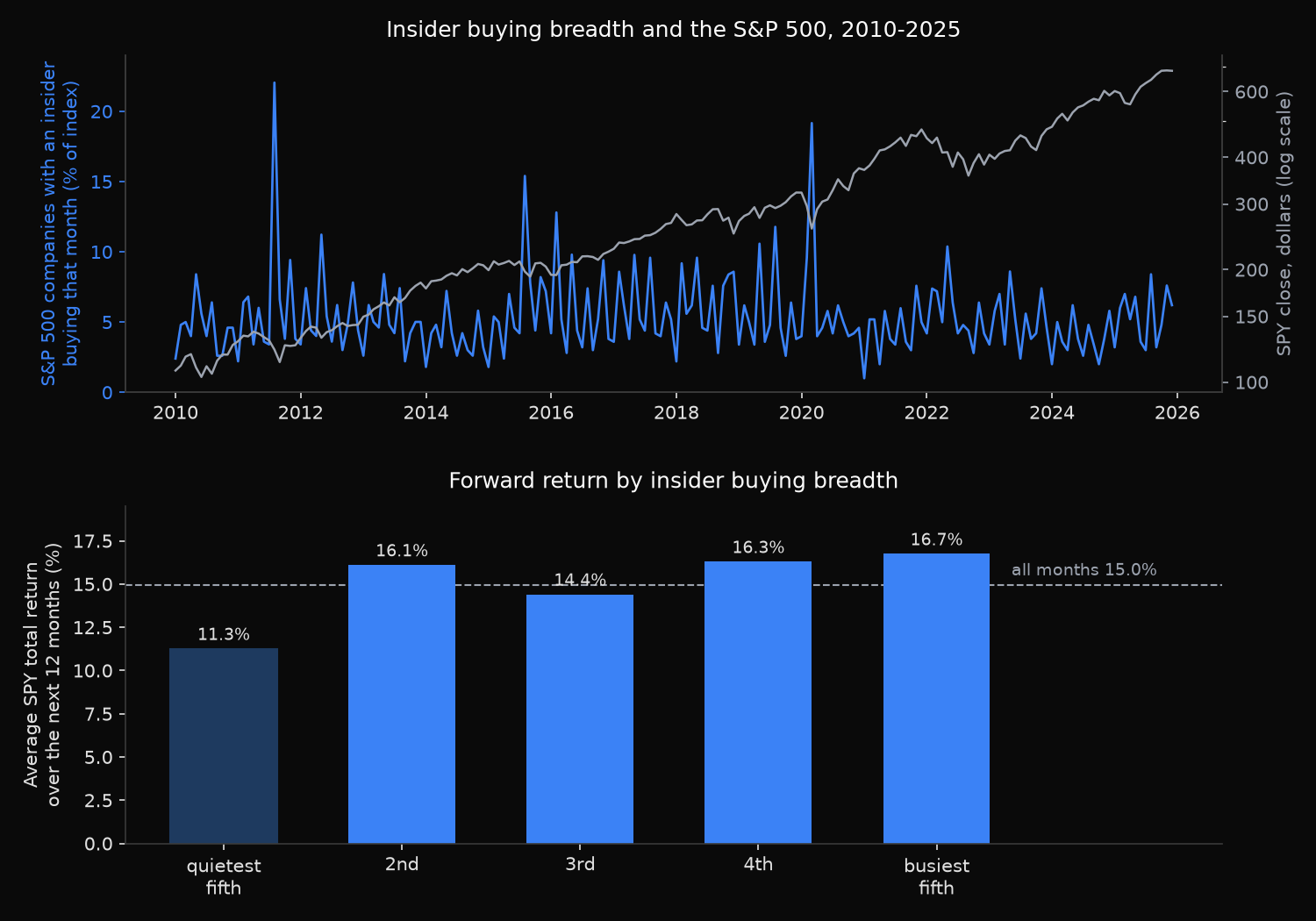
=== S&P 500 insider buying breadth vs the index’s own forward return ===
Signal months: 2010-01 to 2025-08  (n=188)
Open-market trades read: 260,333  (5,149 buyer-months, 37,478 seller-months)
Buy breadth: mean 5.36%  median 4.70%  range 1.00% to 22.04%
Sell breadth: mean 39.09%
Unconditional forward 12-month SPY return: 14.96%

Forward SPY total return by buy-breadth quintile
 quintile  months    breadth range   fwd 3m   fwd 6m   fwd 12m   12m up
        1      38    1.00% -  3.40%    3.85%    6.54%    11.26%    86.8%
        2      40    3.41% -  4.21%    2.91%    7.78%    16.11%    92.5%
        3      37    4.39% -  5.19%    3.97%    6.36%    14.41%    91.9%
        4      36    5.20% -  7.00%    3.49%    8.10%    16.30%    88.9%
        5      37    7.19% - 22.04%    3.67%    7.39%    16.75%    91.9%
          top fifth minus bottom fifth, 12 months: +5.48 points

Newey-West regression of forward return on buy breadth
  horizon  3m  n=188  slope=+0.00190 per point of breadth  t=+1.11  p=0.2677  R2=0.007
  horizon  6m  n=188  slope=+0.00290 per point of breadth  t=+1.07  p=0.2843  R2=0.009
  horizon 12m  n=188  slope=+0.00790 per point of breadth  t=+2.39  p=0.0169  R2=0.034
  sell breadth, 12m  n=188  slope=-0.00173  t=-2.69  p=0.0072  R2=0.022

Excluding 2020 signal months: bottom fifth 11.26%, top fifth 15.22%, spread +3.95 points
Five busiest months for insider buying: 2011-08 (22.0%), 2020-03 (19.2%), 2015-08 (15.4%), 2016-02 (12.8%), 2019-08 (11.8%)

What this tells us

At three and six months there is nothing. The t-statistics are 1.11 and 1.07, and the quintile columns do not order: the second-quietest fifth posts the weakest three-month return of the five.

The twelve-month horizon does produce a signal, and it survives the correction for overlapping windows at t = 2.39. It is small. An R-squared of 0.034 means breadth accounts for roughly 3% of the following year’s return variation, and the ladder is not monotone: the second quintile at 16.11% beats the third at 14.41%.

The information sits at one end. Months in the quietest fifth, where fewer than one company in 29 saw an insider buy, were followed by an average 11.26% over the next year against 14.96% for all months. The other four quintiles fall in a band from 14.41% to 16.75%, which 188 overlapping observations cannot separate. The finding is therefore not that heavy insider buying is bullish; it is that a persistently quiet insider base has preceded a below-average year.

The busiest months explain most of the rest. August 2011, March 2020, August 2015 and February 2016 are the debt-ceiling downgrade, the pandemic crash and two growth scares. Insiders buy in numbers after prices have already fallen, so breadth acts mostly as a coincident gauge of how far the market has dropped, and the strong year that follows is the usual recovery rather than foresight. Removing 2020 alone cuts the top-minus-bottom spread from 5.48 points to 3.95. Selling breadth is the mirror image at t = -2.69.

So what?

Aggregate insider activity belongs in the slow-moving part of a research process, beside valuation and credit spreads, rather than in the entry logic of a strategy. The quarterly and semi-annual horizons that most tactical allocation runs on show no usable relationship.

Where it earns attention is the downside. A stretch of months in which almost nobody inside the largest companies is buying has been the one condition in this sample associated with a materially below-average year, and it is visible in real time. Watching the quiet is more useful than waiting for the wave.

Two requirements follow for anyone rebuilding the series. Standard errors have to be corrected for the overlap, because a twelve-month forward return sampled monthly reuses eleven twelfths of its window. Membership has to be point-in-time and keyed on a company identifier, because insider buying concentrates in companies in trouble, and those are exactly the ones a current roster has already dropped.