Does the Base-Metals-to-Gold Ratio Lead Cyclical Stocks? Signal Test in Python

June 18, 2026

What's the question?

Base metals are tied to industrial demand. Gold is more closely associated with real rates, inflation hedging, and defensive demand. The ratio of base metals to gold is therefore often treated as a compact cyclical signal. When base metals outperform gold, the market may be pricing stronger growth. When gold outperforms base metals, the market may be pricing caution.

The practical question is whether this ratio actually helps forecast equity returns. A plausible macro story is not enough. The signal must be tested against forward returns.

The question is whether a rising DBB/GLD ratio leads stronger subsequent returns for cyclically exposed equities.

The approach

The signal is the six-month change in DBB divided by GLD. The forward returns are measured for XLI, XLB, and SPY. Built from SEC EDGAR public filings and market data, the test uses ten years of monthly observations.

1. Pull ten years of daily prices and returns for DBB, GLD, XLI, XLB, and SPY
2. Convert daily data to complete monthly observations
3. Compute the six-month percentage change in DBB/GLD
4. Sort each monthly signal into quintiles
5. Measure average next-three-month returns for XLI, XLB, and SPY

XLI and XLB are included because industrials and materials should be more sensitive to cyclical commodity signals than the broad market.

Code

import xfinlink as xfl
import pandas as pd
import numpy as np

xfl.set_api_key("YOUR_API_KEY")  # free at https://xfinlink.com/signup

tickers = ["DBB", "GLD", "XLI", "XLB", "SPY"]
prices = xfl.prices(tickers, period="10y", fields=["adj_close", "return_daily"])

price_daily = prices.pivot_table(index="date", columns="ticker", values="adj_close").dropna()
return_daily = prices.pivot_table(index="date", columns="ticker", values="return_daily").dropna()

monthly_prices = price_daily.resample("ME").last()
monthly_returns = (1 + return_daily).resample("ME").prod() - 1

signal = (monthly_prices["DBB"] / monthly_prices["GLD"]).pct_change(6)
forward_spy = (1 + monthly_returns["SPY"]).rolling(3).apply(np.prod, raw=True).shift(-3) - 1

analysis = pd.DataFrame({"signal": signal, "forward_spy": forward_spy}).dropna()
analysis["quintile"] = pd.qcut(analysis["signal"], 5)

print(analysis.groupby("quintile", observed=False)["forward_spy"].mean())

Full script with formatting and visualisation: base-metals-gold-cyclical-signal-python.py

Output

=== Base-Metals-to-Gold Cyclical Signal ===
Signal: 6-month change in DBB/GLD
Forward return window: next 3 months
Sample: 2016-12-31 to 2026-02-28 (111 monthly observations)
Latest signal:  +9.9% (Q5 strongest)

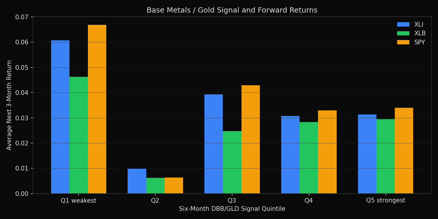
Average next 3-month returns by signal quintile:
Q1 weakest    n=23  XLI= +6.1%  XLB= +4.6%  SPY= +6.7%
Q2            n=22  XLI= +1.0%  XLB= +0.6%  SPY= +0.6%
Q3            n=22  XLI= +3.9%  XLB= +2.5%  SPY= +4.3%
Q4            n=22  XLI= +3.1%  XLB= +2.8%  SPY= +3.3%
Q5 strongest  n=22  XLI= +3.1%  XLB= +3.0%  SPY= +3.4%

Strong-minus-weak signal spread:
XLI spread= -2.9%
XLB spread= -1.7%
SPY spread= -3.3%

What this tells us

The result does not support a simple pro-cyclical interpretation. The weakest DBB/GLD signal quintile had the strongest forward returns: XLI averaged +6.1%, XLB averaged +4.6%, and SPY averaged +6.7% over the next three months.

The strongest signal quintile was still positive, but it did not lead. Q5 averaged +3.1% for XLI, +3.0% for XLB, and +3.4% for SPY. The strong-minus-weak spreads were negative across all three assets.

This pattern is closer to a contrarian signal than a trend-confirmation signal. When base metals have already outperformed gold sharply, part of the cyclical optimism may already be priced. When the ratio is weak, forward returns have historically been stronger in this sample.

So what?

The base-metals-to-gold ratio is useful, but not as a direct buy signal for cyclicals. A rising ratio may confirm improving cyclical sentiment, yet the forward-return evidence does not justify chasing that move mechanically.

For market timing, the better use is conditional. A weak ratio can identify periods when cyclicals are out of favor and forward returns may be more attractive. A strong ratio can confirm the macro backdrop, but it should be paired with valuation, earnings revisions, or momentum breadth before increasing risk.

Built with xfinlink — free financial data API for Python. pip install xfinlink