Do Insider Buying Clusters Predict Returns? Signal Testing in Python

July 26, 2026

What's the question?

Corporate insiders must file a Form 4 with the SEC before the end of the second business day after trading their own company’s stock, and every filing is public. A chief executive buying shares with personal money is making a costly, visible bet that the market has the price wrong.

The version of this idea that circulates most widely is about agreement rather than any single purchase. One director buying could be rebalancing, an option lapsing, or a lawyer suggesting the optics would help after a bad quarter. Four insiders buying in the same month is harder to explain away. That is the cluster hypothesis, and it is testable: company-months with several insiders buying should beat company-months with one.

Size is the competing measure, since one officer committing a large sum may say more than four directors each buying a token amount. Excess return below means the stock’s total return over the three months after the signal, minus SPY over the same window.

The approach

The sample is the S&P 500 from January 2015 to December 2025, on point-in-time membership. Companies removed after a collapse stay in for the months they were actually members, which matters because insider buying spikes when a company is in trouble.

1. Rebuild the roster as of 1 January each year, keyed on company identifier rather than ticker, since symbols get reassigned and recycled. That gives 696 tickers.
2. Pull every open-market purchase (Form 4 code P). Grants, option exercises, and tax withholding are compensation mechanics, not a decision to buy.
3. Drop 10% owners, whose strategic stakes would dominate any dollar-weighted measure, and drop trades under $10,000.
4. Aggregate to company-months on the filing date, so the signal uses only information the public had.
5. Measure the forward three-month total return starting the month after the filing month, and subtract SPY.
6. Winsorise that excess return at the 1st and 99th percentiles, because three-month single-stock returns have long tails.

Purchase size is scaled by market capitalisation, so $2m at a $5bn company ranks above the same $2m at a $500bn company. Significance is assessed on the monthly cross-sectional averages with Newey-West standard errors at three lags, since the overlapping windows would otherwise inflate every t-statistic.

Code

import numpy as np
import pandas as pd
import statsmodels.api as sm
import xfinlink as xfl

xfl.set_api_key("YOUR_API_KEY")  # free at https://xfinlink.com/signup

HORIZON, MIN_TRADE = 3, 10_000
OFFICER_KEYS = ("CEO", "CFO", "COO", "CTO", "President", "Officer", "General Counsel")

def chunked(fn, tickers, size=50, **kw):
    return pd.concat([fn(tickers[i:i + size], **kw)
                      for i in range(0, len(tickers), size)], ignore_index=True)

# point-in-time membership, keyed on company identifier rather than ticker
rosters = {y: xfl.index("sp500", as_of=f"{y}-01-01", limit=600) for y in range(2015, 2027)}
snaps = {y: set(r["entity_id"]) for y, r in rosters.items()}
universe = sorted(set().union(*[set(rosters[y]["ticker"].dropna()) for y in range(2015, 2026)]))

buys = chunked(xfl.insiders, universe, transaction_type="open_market_buy",
               start="2015-01-01", end="2025-12-31", max_rows=300_000)
buys = buys[~buys["insider_role"].isin(("10% Owner", "Other"))]
buys = buys[buys["transaction_value"] >= MIN_TRADE]
buys["month"] = buys["filing_date"].dt.tz_localize(None).dt.to_period("M")
# word boundaries matter: a substring test scores "Director" as an officer,
# because "direCTOr" contains "CTO"
buys["is_officer"] = buys["insider_role"].str.contains(
    r"(?:" + "|".join(OFFICER_KEYS) + r")", case=False, regex=True)

sig = buys.groupby(["entity_id", "month"]).agg(
    ticker=("ticker", "last"),
    n_insiders=("insider_name", "nunique"),
    dollars=("transaction_value", "sum"),
    officer_share=("is_officer", "mean")).reset_index()
sig = sig[[e in snaps[m.year] for e, m in zip(sig["entity_id"], sig["month"])]]

px = chunked(xfl.prices, sorted(sig["ticker"].unique()) + ["SPY"],
             start="2015-01-01", end="2026-07-01", interval="1mo",
             fields=["close", "return_daily", "shares_outstanding"], max_rows=300_000)
px["month"] = px["date"].dt.to_period("M")
px = px.drop_duplicates(["entity_id", "month"]).sort_values(["entity_id", "month"])

# forward 3-month total return, starting the month AFTER the signal month
def fwd(s):
    r = np.log1p(s)
    return np.expm1(r.shift(-1).rolling(HORIZON).sum().shift(-(HORIZON - 1)))

px["fwd"] = px.groupby("entity_id")["return_daily"].transform(fwd)
spy = px[px["ticker"] == "SPY"].set_index("month")["fwd"]

sig = sig.merge(px[["entity_id", "month", "fwd", "close", "shares_outstanding"]],
                on=["entity_id", "month"], how="left")
sig["abn"] = sig["fwd"] - sig["month"].map(spy)
sig["intensity_bp"] = 10_000 * sig["dollars"] / (sig["close"] * sig["shares_outstanding"])
sig = sig.dropna(subset=["abn", "intensity_bp"])
sig["abn"] = sig["abn"].clip(*sig["abn"].quantile([0.01, 0.99]))

sig["bucket"] = np.where(sig["n_insiders"] >= 3, "3+ insiders",
                  np.where(sig["n_insiders"] == 2, "2 insiders", "1 insider"))
sig["size_q"] = "Q" + (sig.groupby("month")["intensity_bp"].rank(pct=True)
                       .mul(4).apply(np.ceil).clip(1, 4).astype(int).astype(str))

# Newey-West t on the time series of monthly cross-sectional means
def nw_t(monthly):
    y = monthly.dropna()
    fit = sm.OLS(y.values, np.ones(len(y))).fit(cov_type="HAC", cov_kwds={"maxlags": HORIZON})
    return fit.tvalues[0]

for key in ["bucket", "size_q"]:
    for name, g in sig.groupby(key):
        monthly = g.groupby("month")["abn"].mean()
        print(f"{name:<12}{len(g):>6}{monthly.mean()*100:>9.2f}%"
              f"{g['abn'].median()*100:>8.2f}%{(g['abn']>0).mean()*100:>8.1f}%{nw_t(monthly):>7.2f}")

# horse race: does headcount survive once size is controlled for?
X = sm.add_constant(pd.DataFrame({"log_n": np.log(sig["n_insiders"]),
                                  "log_intensity": np.log(sig["intensity_bp"])}))
fit = sm.OLS(sig["abn"].values, X).fit(cov_type="cluster",
                                       cov_kwds={"groups": sig["month"].astype(str)})
print(fit.summary())

Full script with formatting and visualisation: insider-buying-clusters-forward-returns-python.py

Output

Point-in-time S&P 500 rosters 2015-2025: 696 distinct tickers
Open-market purchases pulled: 15,830 rows, 626 tickers
After dropping 10% owners and trades under $10,000: 8,311 rows
Firm-months with qualifying insider buying: 2,729
Monthly price coverage of signal companies: 99.2%
Firm-months with a complete 3-month forward window: 2,699
Formation months: 2015-01 to 2026-03
Excess return winsorised at -36.4% / 41.0%; sample mean moves from -0.20% to -0.21%

=== Forward 3-month return vs SPY, S&P 500 insider open-market buys ===
Baseline: all 2,699 firm-months across 135 formation months  mean abnormal -0.44%  NW t -0.79

By number of distinct insiders buying in the filing month
bucket                     n  months   mean abn   median  hit rate    NW t
1 insider              2,160     135     -0.46%   -0.36%     48.6%   -0.79
2 insiders               340     105      0.01%    0.62%     51.5%    0.01
3+ insiders              199      89     -1.43%   -1.03%     48.2%   -1.10

By purchase intensity (dollars bought / market cap), ranked within month
size_q                     n  months   mean abn   median  hit rate    NW t
Q1                       625     132     -0.96%   -0.59%     48.0%   -1.42
Q2                       690     134      0.23%    0.07%     50.3%    0.38
Q3                       656     132     -1.34%   -0.51%     48.8%   -1.57
Q4                       728     135      0.23%   -0.60%     48.6%    0.27

Clusters (3+) by who was buying
who                        n  months   mean abn   median  hit rate    NW t
At least one officer     143      66     -2.43%   -2.20%     46.2%   -1.78
Directors only            56      42     -0.58%    0.97%     53.6%   -0.30

Pooled regression, abnormal return on both measures (SE clustered by month)
  log_n           coef -0.0021   t -0.24   p 0.806
  log_intensity   coef +0.0016   t +0.86   p 0.390
  n = 2,699   R-squared = 0.0004

What this tells us

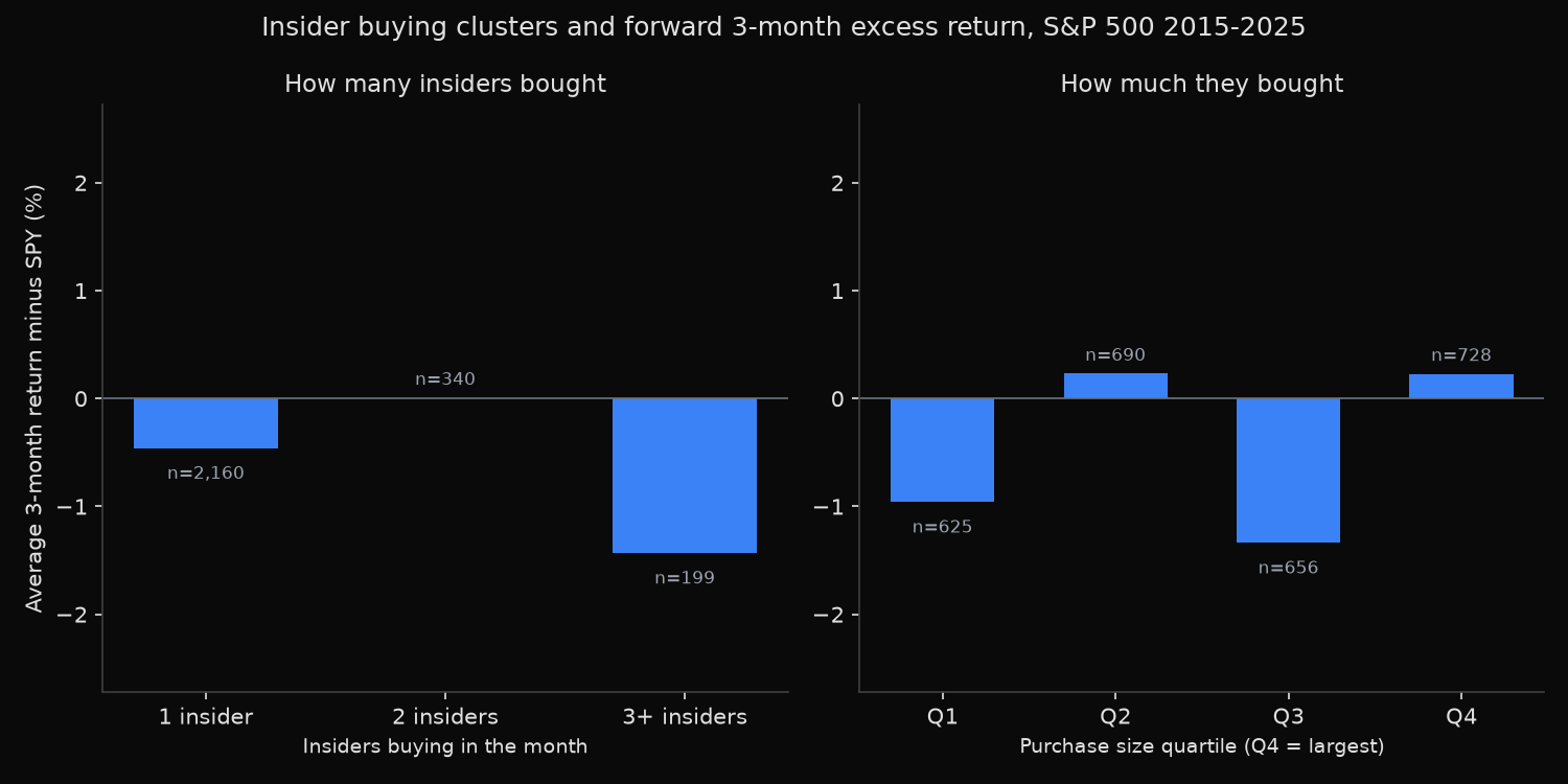
The cluster hypothesis fails. Company-months with three or more distinct insiders buying returned −1.43% versus the market over the next three months, against −0.46% for months with a single buyer. The ordering runs the wrong way, and neither figure is distinguishable from zero.

Purchase size fails in a more instructive shape. The quartile averages run −0.96%, +0.23%, −1.34%, +0.23% across Q1 to Q4, which alternates rather than trends. If dollar intensity carried information the quartiles would line up in order.

Neither measure survives the regression. Excess return on the log of both at once gives a coefficient on headcount of −0.0021 (t of −0.24) and on intensity of +0.0016 (t of +0.86), with an R-squared of 0.0004. Across 2,699 company-months the two variables jointly explain effectively none of the variation in what happens next.

The cell closest to significance points the opposite way from the folklore: clusters including at least one officer returned −2.43% at a t-statistic of −1.78. As a standalone claim that would be data mining, one cell out of roughly a dozen examined. What it establishes is that no configuration of the signal produced the positive result the hypothesis predicts.

The universe explains most of the gap between this and the published academic work. Insider buying earns its reputation from studies dominated by small and micro-cap firms, where coverage is thin and managers genuinely know things the market does not; every company here is followed by dozens of analysts.

Selection runs against the signal too, because insiders buy after prices fall and keep buying into declines that continue. Every open-market purchase in the sample averaged −0.44% against SPY over the following quarter, at a hit rate near 48%. Large-cap insider buying is, on average, early.

So what?

Do not build a screen that ranks large-cap stocks by how many insiders bought last month. The variable does not rank anything: 199 cluster months over eleven years produced a slightly worse outcome than the 2,160 single-buyer months.

Treat the result as a boundary rather than a prohibition. Insider buying is not dead everywhere; its value depends on a market being inattentive, and the S&P 500 is the least inattentive market that exists. Run the same code against small caps, where the information asymmetry survives. Substituting a different index in the roster call is a one-line change.

A cluster still marks a company where something has already gone wrong, since the buying follows the drawdown rather than leading the recovery. That earns it a place as a prompt to read the filings, not as a reason to own the stock.

Anyone holding a backtest where this signal works should check three things: whether the universe was survivorship-filtered, whether the signal was dated to the transaction rather than the filing, and whether the t-statistics treated overlapping windows as independent. Each alone can manufacture significance from a series that has none.

Built with xfinlink — free financial data API for Python. pip install xfinlink