
What’s the question?
A price gap is the distance between one session’s closing price and the next session’s opening price. Trading stops, news arrives, and the stock reopens away from where it left off. How much of a stock’s long-run return accrues in that closed-market interval is split out in an overnight versus intraday decomposition.
Technical analysis holds that gaps get filled: price returns to the prior close, because the gap is an unbalanced move the market corrects. Published fill rates land between 60 and 90 percent.
The measurement has no control group. A price that wanders at random will also cross back over its prior close sooner or later, and the wider its daily range, the sooner. What settles the argument is the fill rate against what a random walk of the same volatility would deliver.
That comparison has a closed form. For a random walk with no drift, the chance of touching a level at some point within N sessions is exactly twice the chance of finishing beyond it, a result known as the reflection principle.
The approach
- Take every member of the S&P 500 as of 2 January 2016 and follow all 500 entities by identity rather than by symbol to the end of 2025, so companies later dropped from the index stay in: 1,100,670 daily bars.
- One company under one symbol is one price series; a symbol change starts a new series rather than splicing two eras together.
- A session is a gap when its open sits 3 to 25 percent from the previous close, on split-adjusted prices. Ex-dividend sessions drop out, and so do moves past 25 percent, where spin-offs and restructurings enter the sample.
- A gap up is filled within N sessions when the lowest traded price over those sessions reaches the prior close, a gap down when the highest price does. The gap session itself counts.
- The random-walk probability is computed twice per event: on the volatility of the 60 sessions before the gap and on the volatility realised over the N sessions measured. A simulation calibrates the formula against a walk observed through daily highs and lows.
Code
import numpy as np
import pandas as pd
import xfinlink as xfl
from scipy.stats import norm

xfl.set_api_key("YOUR_API_KEY")  # free at https://xfinlink.com/signup

roster = xfl.index("sp500", as_of="2016-01-01")
px = xfl.prices(entity_id=sorted(int(i) for i in roster["entity_id"]),
                start="2016-01-01", end="2025-12-31",
                fields=["open", "high", "low", "close", "adj_close", "dividend"])

rows = []
for (eid, tk), g in px.groupby(["entity_id", "ticker"]):
    g = g.sort_values("date")
    f = (g["adj_close"] / g["close"]).to_numpy()      # split factor for that bar
    o, h, lo = (g[k].to_numpy() * f for k in ("open", "high", "low"))
    c = g["adj_close"].to_numpy()
    prev_c = np.concatenate([[np.nan], c[:-1]])
    gap = o / prev_c - 1.0
    logret = np.diff(np.log(c), prepend=np.nan)

    i0 = np.arange(len(c))
    ok = ((np.abs(gap) >= 0.03) & (np.abs(gap) <= 0.25)
          & pd.isna(g["dividend"]).to_numpy() & (i0 >= 60) & (i0 <= len(c) - 60))
    for i in np.where(ok)[0]:
        seg = np.concatenate([[np.log(c[i] / o[i])],
                              np.log(c[i + 1:i + 60] / c[i:i + 59])])
        r = {"up": gap[i] > 0, "open": o[i], "prev_c": prev_c[i],
             "sig_pre": logret[i - 60:i].std(ddof=1)}
        for N in (5, 20, 60):
            r[f"fill{N}"] = (lo[i:i + N].min() <= prev_c[i] if gap[i] > 0
                             else h[i:i + N].max() >= prev_c[i])
            r[f"sig{N}"] = seg[:N].std(ddof=1)
        rows.append(r)

ev = pd.DataFrame(rows)

def rw(d, N, sig):   # reflection principle: chance of touching the prior close
    return 2 * norm.cdf(-np.abs(np.log(d["open"] / d["prev_c"])) / (d[sig] * np.sqrt(N)))

for lab, sub in [("gap up", ev[ev["up"]]), ("gap down", ev[~ev["up"]])]:
    for N in (5, 20, 60):
        print(f"{lab:9}{N:3}d  filled {sub[f'fill{N}'].mean():.3f}  "
              f"random walk {rw(sub, N, f'sig{N}').mean():.3f}")
Full script with formatting and visualisation: do-price-gaps-get-filled-random-walk-python.py
Output
==============================================================================
Do opening price gaps get filled?  S&P 500 roster of 2 January 2016, followed to 2025
527 price series, 1,100,670 daily bars, 26,863 gaps of 3% to 25%
==============================================================================

Estimator check: simulated driftless random walk, 26 steps a session, 40,000 paths
  barrier  daily vol  sessions   formula  simulated
     3.0%       2.0%         5     0.502      0.468
     5.0%       2.0%        20     0.576      0.561
    10.0%       3.0%        20     0.456      0.440
     5.0%       2.0%        60     0.747      0.739

GAP UP   n = 13,397   median gap 4.32%   filled same session 0.219
 sessions   filled   RW, trailing vol   RW, realised vol
        5    0.485              0.476              0.431
       20    0.640              0.689              0.663
       60    0.742              0.809              0.788

GAP DOWN   n = 13,466   median gap 4.28%   filled same session 0.185
 sessions   filled   RW, trailing vol   RW, realised vol
        5    0.455              0.394              0.471
       20    0.663              0.624              0.673
       60    0.809              0.765              0.786

Filled within 20 sessions, by gap size
                    gap up                           gap down
    size      n  filled   trail    real         n  filled   trail    real
    3-5%   8436   0.708   0.750   0.722      8478   0.723   0.711   0.736
    5-8%   3494   0.570   0.639   0.612      3291   0.605   0.550   0.625
   8-12%   1037   0.455   0.517   0.503      1118   0.538   0.390   0.512
  12-25%    430   0.323   0.308   0.320       579   0.349   0.225   0.341

Filled within 20 sessions, by year
  year      n      up     RW    down     RW
  2016   1371   0.495  0.538   0.652  0.536
  2017    980   0.444  0.433   0.465  0.428
  2018   1416   0.648  0.569   0.530  0.556
  2019   1315   0.508  0.514   0.551  0.540
  2020  11006   0.705  0.757   0.713  0.791
  2021   1670   0.687  0.665   0.681  0.623
  2022   3194   0.662  0.692   0.716  0.703
  2023   1594   0.556  0.572   0.569  0.555
  2024   1889   0.526  0.539   0.606  0.528
  2025   2428   0.635  0.627   0.687  0.669

Return from the gap open, net of the universe median over the same dates
            20d median  share > 0  60d median  share > 0
gap up           0.06%      0.503       1.07%      0.527
gap down        -0.44%      0.481       0.61%      0.517
What this tells us
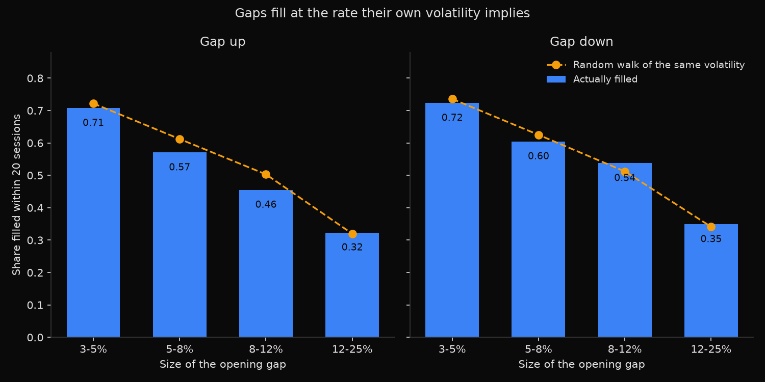
The folklore fill rate holds up. Within 20 sessions 64.0 percent of gaps up and 66.3 percent of gaps down return to the prior close, and by 60 sessions the figures reach 74.2 and 80.9 percent.
The benchmark column removes that reading. A random walk carrying each stock’s own realised volatility fills 66.3 percent of the gaps up and 67.3 percent of the gaps down over 20 sessions, 78.8 and 78.6 percent over 60. Observed and benchmark are never more than 5.4 points apart in any cell, and the simulation shows the formula runs 0.8 to 3.4 points high against the way the fill is actually measured, which covers most of what separates them.
Gaps fill because prices move, and a wider gap takes longer to walk back across. The trailing-volatility column shows what that costs a forecaster: for gaps down it falls further below the observed rate the larger the gap, reaching 39.0 percent predicted against 53.8 percent observed at 8 to 12 percent and 22.5 against 34.9 at 12 to 25 percent, because volatility after a downside gap runs above the volatility before it.
Gap events cluster in stressed markets, 11,006 of the 26,863 falling in 2020 alone, and yearly fill rates run from 44 to 72 percent. The sign of the miss changes from year to year, which is what a null result looks like.
Nor does a gap say much about the following month. Net of the universe over the same dates, the median 20-session return after a gap up is 0.06 percent, with 50.3 percent of events positive; after a gap down it is negative 0.44 percent, with 48.1 percent positive.
So what?
Fading a gap and waiting for the fill is not a mean-reversion trade. It is a bet that a volatile stock will trade through a nearby level, and it collects nothing for being right, because the volatility that produces the fill produces the adverse excursion beforehand. The 12 to 25 percent bucket makes the arithmetic plain: two thirds of those gaps never fill within a month, so the trade wins small and often and loses large and rarely.
The fill probability does have a use, and it is not directional. Read as a barrier-touch estimate, it prices the odds that a stop or a limit resting at the old close gets hit before a chosen horizon. Use realised volatility for that, and treat a trailing-volatility estimate as a floor after a downside gap.
Built with xfinlink — free financial data API for Python.