How Much Drawdown Does Month-End Data Hide? Sampling Frequency and Maximum Drawdown in Python

September 4, 2026

What’s the question?

Maximum drawdown is the largest peak-to-trough fall in a price series. Most investors read it as the answer to a single question: how bad did this get. It is also the risk statistic most sensitive to something almost nobody reports alongside it, which is how often the price was sampled.

A monthly series carries twelve observations a year, so a trough that arrives on the 12th and is half recovered by the 30th leaves no mark on it at all. Fund factsheets and most academic return datasets quote drawdowns computed from month-end prices, because that is the frequency the underlying data arrives in. Daily prices see every trough. The gap between those two answers is measurable.

The approach

1. Take S&P 500 membership as it stood on 31 December 2019 and keep every fifth company in identifier order. That fixes a 101-name sample before the measurement window opens, on a rule unrelated to what the prices then did.
2. Pull daily split-adjusted closes from 2020 through 2024, keyed on the company identifier rather than the ticker symbol, so a company that changed symbol inside the window keeps one continuous series. Six names stop early because they were acquired or merged; their history counts as far as it runs.
3. Rebuild each series on three grids: every trading day, the last close of each week, the last close of each month.
4. Compute the maximum drawdown on each grid, then measure what share of the daily depth the coarser grids recover.

Drawdowns here are price drawdowns, computed on split-adjusted closes with dividends excluded. SPY sits in the sample as an index reference, and the 2020-2024 window is chosen because it contains one violent crash and one slow bear market, which turn out to behave very differently.

Code

import pandas as pd
import xfinlink as xfl

xfl.set_api_key("YOUR_API_KEY")  # free at https://xfinlink.com/signup

START, END = "2020-01-01", "2024-12-31"

roster = xfl.index("sp500", as_of="2019-12-31")
ids = sorted(roster["entity_id"].tolist())[::5]

frames = [xfl.prices(entity_id=ids[i:i + 20], start=START, end=END,
                     fields=["adj_close"], max_rows=100000)
          for i in range(0, len(ids), 20)]
px = pd.concat(frames + [xfl.prices("SPY", start=START, end=END,
                                    fields=["adj_close"])], ignore_index=True)


def drawdown(s):
    return s / s.cummax() - 1


def episode(s):
    d = drawdown(s)
    trough = d.idxmin()
    return s[:trough].idxmax(), trough, d.min()


rows, series = [], {}
for eid, g in px.groupby("entity_id"):
    s = g.set_index("date")["adj_close"].sort_index().dropna()
    if len(s) < 500:
        continue
    week, month = s.resample("W-FRI").last().dropna(), s.resample("ME").last().dropna()
    series[g["ticker"].iloc[-1]] = (s, month)
    rows.append({"ticker": g["ticker"].iloc[-1], "days": len(s),
                 "daily": drawdown(s).min(), "weekly": drawdown(week).min(),
                 "monthly": drawdown(month).min()})

dd = pd.DataFrame(rows)
dd["hidden_pp"] = (dd["monthly"] - dd["daily"]) * 100
dd["captured"] = dd["monthly"] / dd["daily"]
stocks = dd[dd["ticker"] != "SPY"]
spy = dd[dd["ticker"] == "SPY"].iloc[0]

print(f"S&P 500 roster of 2019-12-31, every 5th name: {len(stocks)} companies, 2020-2024")
print(f"full five-year price history: {(stocks['days'] == 1258).sum()}")
print()
print("                     daily   weekly   month-end")
print("median max drawdown %6.1f%% %7.1f%% %10.1f%%" % (
    stocks["daily"].median() * 100, stocks["weekly"].median() * 100,
    stocks["monthly"].median() * 100))
print("median depth captured        %7.3f %10.3f" % (
    (stocks["weekly"] / stocks["daily"]).median(), stocks["captured"].median()))
print()
print("month-end understatement (pp): median %.1f  90th pct %.1f  max %.1f" % (
    stocks["hidden_pp"].median(), stocks["hidden_pp"].quantile(0.9),
    stocks["hidden_pp"].max()))
print("names hiding more than 10pp: %d of %d" % (
    (stocks["hidden_pp"] > 10).sum(), len(stocks)))
print()
s, month = series["SPY"]
p_d, t_d, v_d = episode(s)
p_m, t_m, v_m = episode(month)
covid = month.loc["2020-03-31"] / month.loc["2020-01-31"] - 1
print("SPY: daily %.1f%%  weekly %.1f%%  month-end %.1f%%" % (
    spy["daily"] * 100, spy["weekly"] * 100, spy["monthly"] * 100))
print("  worst daily episode      %s to %s  %.1f%%" % (p_d.date(), t_d.date(), v_d * 100))
print("  worst month-end episode  %s to %s  %.1f%%" % (p_m.date(), t_m.date(), v_m * 100))
print("  2020 crash on the month-end grid                  %.1f%%" % (covid * 100))
print()
print("widest month-end gaps")
for _, r in stocks.nlargest(5, "hidden_pp").iterrows():
    print("  %-5s daily %.1f%%  month-end %.1f%%  hidden %.1fpp" % (
        r["ticker"], r["daily"] * 100, r["monthly"] * 100, r["hidden_pp"]))

Full script with formatting and visualisation: max-drawdown-sampling-frequency-python.py

Output

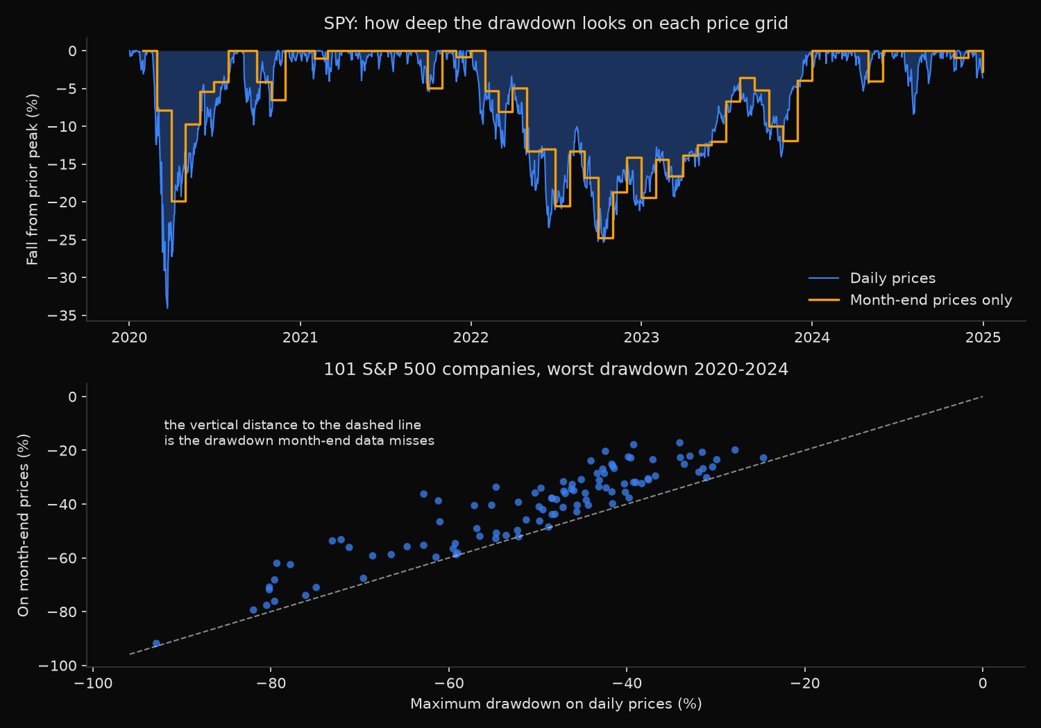
S&P 500 roster of 2019-12-31, every 5th name: 101 companies, 2020-2024
full five-year price history: 95

                     daily   weekly   month-end
median max drawdown  -47.2%   -45.1%      -37.9%
median depth captured          0.960      0.813

month-end understatement (pp): median 8.3  90th pct 16.8  max 26.6
names hiding more than 10pp: 41 of 101

SPY: daily -34.1%  weekly -32.2%  month-end -24.8%
  worst daily episode      2020-02-19 to 2020-03-23  -34.1%
  worst month-end episode  2021-12-31 to 2022-09-30  -24.8%
  2020 crash on the month-end grid                  -19.9%

widest month-end gaps
  LYB   daily -62.8%  month-end -36.3%  hidden 26.6pp
  LKQ   daily -61.2%  month-end -38.8%  hidden 22.4pp
  PWR   daily -42.4%  month-end -20.4%  hidden 22.0pp
  GWW   daily -39.2%  month-end -17.9%  hidden 21.3pp
  PH    daily -54.7%  month-end -33.7%  hidden 21.0pp

What this tells us

Month-end prices recover 81.3% of the daily drawdown depth at the median, which leaves 8.3 percentage points unrecorded for a typical large-cap company. Weekly closes recover 96.0%, giving up only 1.7 points. The loss is therefore not proportional to the sampling interval. A week rarely closes far from its own low, while a month contains about 21 closes and the odds that the worst of them is also the last one are slim. Exactly one name in the sample, SBAC, bottomed on a month-end and lost nothing.

The damage is concentrated in fast declines. LYB fell 62.8% on daily prices and shows 36.3% on month-end prices, because the March 2020 bottom arrived on the 23rd and a large part of it was already recovered by the 31st. Every name in the top five of that table has the same story, and the 41 companies hiding more than 10 points are mostly cyclicals whose worst episode was the crash rather than the 2022 decline.

SPY makes the sharpest version of the point, because changing the grid changes which episode looks worst rather than only how deep it looks. On daily prices the worst SPY drawdown is the crash from 19 February to 23 March 2020, at 34.1%. On month-end prices that same crash reads 19.9%, and the worst drawdown instead becomes the grinding fall from December 2021 to September 2022, at 24.8%. A nine-month decline fits a month-end grid almost perfectly. A five-week one does not.

So what?

A drawdown figure without its sampling frequency attached cannot be compared with anything. A fund reporting monthly max drawdown against a benchmark drawdown computed from daily prices wins part of that comparison before either series is examined, and the advantage is worth roughly 8 points on this evidence, more when the market breaks quickly. Match the grids first, then compare.

For risk limits and stop rules the daily figure is the one that binds, since margin calls, redemptions, and the urge to sell all arrive on the day the loss is real rather than at the end of the month. Backtests deserve the same treatment: a monthly-rebalanced strategy marked only at month-end will report a drawdown no investor holding it actually lived through, and the error is largest in exactly the periods that determine whether the strategy survives.

Where only monthly data exists, treat the drawdown it produces as a floor rather than an estimate. Scaling it up by the 0.813 median from this sample is a rough correction and nothing more, since the individual ratios run from 0.46 to 1.00. Daily prices remove the guess.

Built with xfinlink — free financial data API for Python. pip install -U xfinlink