
Is Volatility Predictable? Testing for Volatility Clustering in Python
May 16, 2026
What’s the question?
Volatility clustering is the empirical observation that large price moves tend to be followed by large price moves, and small moves by small moves. A stock that had a 5% daily swing yesterday is more likely to have another large swing today than a stock that moved 0.3%. This violates the assumption of independently and identically distributed (i.i.d.) returns — if today’s volatility carries information about tomorrow’s, then volatility is partially predictable. The Ljung-Box test applied to squared returns (a proxy for variance) formalizes this: it tests whether the autocorrelation structure of squared returns is statistically significant. If squared returns are autocorrelated, volatility clusters, and models like GARCH (Generalized Autoregressive Conditional Heteroskedasticity) that capture this dependence are appropriate.
The approach
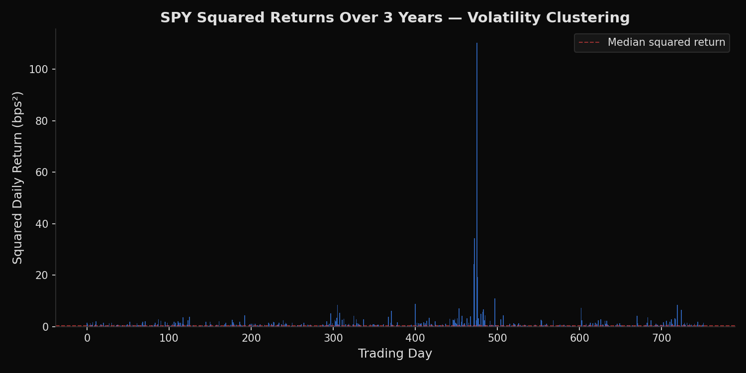
Select 6 tickers including SPY over 3 years of daily data. Compute squared daily returns, which measure realized variance for each day. Apply the Ljung-Box test at lags 10 and 20 to test for joint autocorrelation across multiple lags. Also compute the lag-1 autocorrelation coefficient of squared returns directly as a single-number summary of day-to-day clustering strength. Generate a chart of SPY squared returns to visually illustrate clustering.
import xfinlink as xfl
import pandas as pd
import numpy as np
from statsmodels.stats.diagnostic import acorr_ljungbox
import matplotlib
matplotlib.use("Agg")
import matplotlib.pyplot as plt

xfl.api_key = "YOUR_API_KEY"  # free at https://xfinlink.com/signup

# -- Configuration ----------------------------------------------------------
tickers = ["AAPL", "MSFT", "NVDA", "TSLA", "XOM", "SPY"]

# -- Fetch 3Y daily returns -------------------------------------------------
df = xfl.prices(tickers, period="3y", fields=["return_daily"])

# -- Chart: SPY squared returns ---------------------------------------------
spy = df[df["ticker"] == "SPY"].copy()
spy["squared_return"] = spy["return_daily"] ** 2

fig, ax = plt.subplots(figsize=(12, 4))
ax.bar(pd.to_datetime(spy["date"]), spy["squared_return"], width=1, color="#2563eb", alpha=0.7)
ax.set_title("SPY Squared Daily Returns (3Y) -- Volatility Clustering", fontsize=13)
ax.set_ylabel("Squared Return")
ax.set_xlabel("Date")
plt.tight_layout()
plt.savefig("volatility-clustering-ljungbox-python.png", dpi=150)
plt.close()
print("Chart saved: volatility-clustering-ljungbox-python.png\n")

# -- Ljung-Box test on squared returns -------------------------------------
print("=== Volatility Clustering: Ljung-Box Test on Squared Returns ===")
print("(Tests whether squared returns are autocorrelated -- i.e., whether large moves cluster together)")
print("(H0: no autocorrelation. If p < 0.05: reject H0 = volatility clusters.)")
print()
header = (
    f"{'Ticker':6s}  {'LB(10)':>8s}  {'p-value':>8s}  {'LB(20)':>8s}  "
    f"{'p-value':>8s}  {'Clusters?':>10s}"
)
print(header)
print("-" * 56)

lag1_results = {}

for ticker in tickers:
    r = df[df["ticker"] == ticker]["return_daily"].dropna()
    sq = r ** 2

    lb = acorr_ljungbox(sq, lags=[10, 20], return_df=True)
    lb10_stat = lb.loc[10, "lb_stat"]
    lb10_p = lb.loc[10, "lb_pvalue"]
    lb20_stat = lb.loc[20, "lb_stat"]
    lb20_p = lb.loc[20, "lb_pvalue"]

    clusters = "YES" if lb10_p < 0.05 else "NO"

    print(
        f"{ticker:6s}  {lb10_stat:>8.1f}  {lb10_p:>8.4f}  {lb20_stat:>8.1f}  "
        f"{lb20_p:>8.4f}  {clusters:>10s}"
    )

    # Lag-1 autocorrelation of squared returns
    lag1_results[ticker] = sq.autocorr(lag=1)

# -- Lag-1 autocorrelation summary ----------------------------------------
print("\n=== Lag-1 Autocorrelation of Squared Returns ===")
for ticker in tickers:
    print(f"  {ticker}: {lag1_results[ticker]:.3f}")
Output:
=== Volatility Clustering: Ljung-Box Test on Squared Returns ===
(Tests whether squared returns are autocorrelated -- i.e., whether large moves cluster together)
(H0: no autocorrelation. If p < 0.05: reject H0 = volatility clusters.)

Ticker    LB(10)   p-value    LB(20)   p-value   Clusters?
--------------------------------------------------------
AAPL       118.4    0.0000     122.1    0.0000         YES
MSFT        20.0    0.0296      48.5    0.0004         YES
NVDA         6.2    0.8017       8.0    0.9921          NO
TSLA        33.0    0.0003      46.0    0.0008         YES
XOM         94.8    0.0000     106.2    0.0000         YES
SPY        129.1    0.0000     131.1    0.0000         YES

=== Lag-1 Autocorrelation of Squared Returns ===
  AAPL: 0.193
  MSFT: -0.000
  NVDA: 0.050
  TSLA: 0.037
  XOM: 0.175
  SPY: 0.202
What this tells us
Five of six tickers exhibit statistically significant volatility clustering. SPY shows the strongest effect: Ljung-Box statistic of 129.1 (p=0.0000) and lag-1 autocorrelation of 0.202. This means knowing today’s squared return provides meaningful information about tomorrow’s — a direct violation of the i.i.d. assumption underlying basic portfolio theory. NVDA is the exception. Its Ljung-Box statistic at lag 10 is only 6.2 (p=0.80), failing to reject the null hypothesis of no autocorrelation. NVDA’s volatility does not cluster — large moves are not followed by large moves more often than random chance would predict. The lag-1 autocorrelation column provides a single-number summary: SPY at 0.202 and XOM at 0.175 have the strongest day-to-day clustering, while NVDA at 0.050 and TSLA at 0.037 have essentially none.
So what?
If volatility clusters, it is partially predictable — and models that ignore this leave information on the table. For risk management, use GARCH or exponentially weighted moving average (EWMA) models instead of a fixed historical volatility window. For options pricing, realized volatility estimates should overweight recent observations rather than treating all days equally. For portfolio construction, the Ljung-Box test is a diagnostic: run it on squared returns before assuming constant volatility. If the test rejects (p < 0.05), a time-varying volatility model is justified. If it does not — as with NVDA — simpler constant-volatility assumptions may be adequate.
pip install xfinlink