
What’s the question?
Beta is the slope from regressing a stock’s returns on the market’s returns. A beta of 1.2 says the stock has moved 1.2 percent for every 1 percent the market moved. That number sets hedge ratios and defines what "market neutral" means on a risk report.
The word "market" hides a choice. In practice it means whichever index sits on the right-hand side of the regression, and the default is capitalisation-weighted, where a company counts in proportion to its size. In a cap-weighted portfolio of 466 S&P 500 members, the largest company ended the window tested here at 8.66 percent of the total. Weight those same 466 companies equally and each one holds 0.21 percent.
Same holdings, different weights. If beta survives the switch, the benchmark is a detail. If it does not, then every hedge ratio and every cost-of-equity estimate carries an assumption nobody wrote down. A guide to why beta differs between sources treats the benchmark as one of four settings that move the estimate, alongside window, return frequency and shrinkage.
The approach
The sample is the S&P 500 as it stood on 5 September 2023, from a point-in-time roster, carried by entity id so that a ticker retired or reassigned later cannot quietly swap one company for another. Of the 500, 466 carry a complete weekly return series through 4 September 2026; names without one leave the sample.
- Pull three years of weekly price returns for every member, 156 observations each.
- Build two markets out of those same companies. The cap-weighted one resets to filed share counts in the opening week of each quarter and lets weights drift with price in between, which is how a capitalisation index actually behaves. The equal-weighted one is the cross-sectional average return, rebalanced weekly.
- Regress each company’s weekly return on each market separately by ordinary least squares. Each company is removed from the market it is measured against, so a company carrying 8 percent of the index does not help explain itself.
- Sort the results by market capitalisation at the start of the window.
Weekly rather than daily returns, for a specific reason: daily betas run low for thinly traded names whose prices react a day late, and that bias would land precisely where this test looks, on the smaller members.
Code
import time
from concurrent.futures import ThreadPoolExecutor

import numpy as np
import pandas as pd
import xfinlink as xfl

xfl.set_api_key("YOUR_API_KEY")  # free at https://xfinlink.com/signup

START, END = "2023-09-05", "2026-09-04"


def retry(fn, *a, **k):
    for attempt in range(5):
        try:
            return fn(*a, **k)
        except Exception:
            if attempt == 4:
                raise
            time.sleep(4 * (attempt + 1))


roster = sorted(xfl.index("sp500", as_of=START)["entity_id"].dropna().astype(int).unique())


def grab(i):
    try:
        return retry(xfl.prices, entity_id=i, start=START, end=END, interval="1w",
                     fields=["return_daily"])
    except Exception:
        return pd.DataFrame(columns=["entity_id", "ticker", "date", "return_daily"])


with ThreadPoolExecutor(4) as ex:
    px = pd.concat(ex.map(grab, roster), ignore_index=True)

R = px.drop_duplicates(["entity_id", "date"]).pivot(index="date", columns="entity_id",
                                                    values="return_daily")
R = R[R.notna().sum(axis=1) >= 0.9 * R.shape[1]]
R = R[R.columns[R.notna().sum() == len(R)]]

resets = list(pd.Series(R.index, index=R.index).groupby([R.index.year, R.index.quarter]).min())
cols = list(R.columns)


def caps_on(d):
    lo = (d - pd.Timedelta(days=10)).strftime("%Y-%m-%d")
    hi = (d + pd.Timedelta(days=6)).strftime("%Y-%m-%d")
    last = lambda m: (m.dropna(subset=["market_cap"]).sort_values("period_end")
                      .groupby("entity_id")["market_cap"].last().to_dict())
    out = {}
    for i in range(0, len(cols), 100):
        out.update(last(retry(xfl.metrics, entity_id=cols[i:i + 100], period_type="daily",
                              fields=["market_cap"], start=lo, end=hi, max_rows=100000)))
    for e in [c for c in cols if c not in out]:
        out.update(last(retry(xfl.metrics, entity_id=int(e), period_type="daily",
                              fields=["market_cap"], start=lo, end=hi)))
    return pd.Series(out)


CAP = pd.DataFrame({d: caps_on(d) for d in resets}).T
CAP = CAP[[c for c in cols if c in CAP.columns]].dropna(axis=1)
R = R[CAP.columns]

# inside a quarter the cap portfolio is buy-and-hold, so weights drift with price
V = pd.DataFrame(index=R.index, columns=R.columns, dtype=float)
VP = V.copy()
for i, d in enumerate(resets):
    upper = resets[i + 1] if i + 1 < len(resets) else R.index[-1]
    seg = R.index[(R.index > d) & (R.index <= upper)]
    c, g = CAP.loc[d].values, np.cumprod(1.0 + R.loc[seg].values, axis=0)
    V.loc[seg], VP.loc[seg] = c * g, c * np.vstack([np.ones(len(c)), g[:-1]])

keep = V.notna().all(axis=1)
Vv, VPv, Rv = V[keep].values, VP[keep].values, R[keep].values
n = Rv.shape[1]

# every company is measured against a market that excludes it
cap_ex = (Vv.sum(1, keepdims=True) - Vv) / (VPv.sum(1, keepdims=True) - VPv) - 1.0
ew_ex = (Rv.sum(1, keepdims=True) - Rv) / (n - 1)


def fit(y, x):
    xm, ym = x - x.mean(0), y - y.mean(0)
    b = (xm * ym).sum(0) / (xm * xm).sum(0)
    r2 = b ** 2 * (xm * xm).sum(0) / (ym * ym).sum(0)
    return b, r2, (ym - b * xm).std(0, ddof=2) * np.sqrt(52)


b_cap, r2_cap, rv_cap = fit(Rv, cap_ex)
b_ew, r2_ew, rv_ew = fit(Rv, ew_ex)

print(f"{n} companies, {len(Rv)} weekly returns")
print(f"beta  cap {b_cap.mean():.3f}  equal {b_ew.mean():.3f}   "
      f"higher against equal weight: {(b_ew > b_cap).mean() * 100:.1f}%")
print(f"R2    cap {r2_cap.mean():.3f}  equal {r2_ew.mean():.3f}")
print(f"residual volatility  cap {rv_cap.mean() * 100:.1f}%  equal {rv_ew.mean() * 100:.1f}%")
print(f"the two markets correlate "
      f"{np.corrcoef(Vv.sum(1) / VPv.sum(1) - 1, Rv.mean(1))[0, 1]:.4f}")
Full script with formatting and visualisation: beta-cap-weighted-vs-equal-weighted-market-python.py
Output
====================================================================================
ONE COMPANY, TWO BETAS: CAP-WEIGHTED AND EQUAL-WEIGHTED MARKETS
====================================================================================
Roster     S&P 500 as at 2023-09-05: 500 companies, of which 466 carry a
           complete weekly return series through 2026-09-04
Sample     156 weekly returns, 2023-09-11 to 2026-08-31
Weights    cap weights reset to filed share counts on 13 quarter-opening weeks,
           drifting with price in between
Betas      ordinary least squares on weekly price returns; each company is dropped
           from the market it is measured against

The two markets, built from the same companies
                                  cap-weighted  equal-weighted
  Total return                          69.76%          54.30%
  Annualised volatility                 14.06%          13.44%
  Largest weight at the end              8.66%           0.21%
  Correlation of the two weekly return series           0.8274

Cross-section of the two betas
                            mean   median     p10     p90
  Beta, cap-weighted       0.783    0.761   0.182   1.378
  Beta, equal-weighted     0.989    0.985   0.434   1.584
  Equal minus cap          0.206    0.238  -0.070   0.453
  Companies whose equal-weighted beta is the higher of the two: 85.8%
  Rank correlation between the two betas: 0.903

Share of a company's return variance the market explains
                            mean   median
  Cap-weighted             0.149    0.127
  Equal-weighted           0.212    0.182
  Companies better explained by the equal-weighted market: 82.2%
  Average annualised risk left after a beta hedge: 28.7% against the cap-weighted market, 27.8% against the equal-weighted one

By market-capitalisation decile at the start of the window
   Dec   n   median cap  beta cap  beta EW   R2 cap   R2 EW  left cap  left EW
     1  47          8bn     0.929    1.295    0.137   0.238     35.8%    33.7%
     2  47         13bn     0.799    1.107    0.137   0.237     32.9%    31.3%
     3  46         16bn     0.811    1.048    0.143   0.224     30.2%    28.9%
     4  47         20bn     0.688    0.941    0.135   0.222     26.4%    25.0%
     5  46         27bn     0.820    1.032    0.166   0.226     27.8%    26.9%
     6  47         35bn     0.652    0.895    0.134   0.208     26.2%    25.1%
     7  46         45bn     0.769    0.917    0.162   0.205     27.0%    26.5%
     8  47         64bn     0.775    0.912    0.151   0.191     27.2%    26.8%
     9  46        111bn     0.794    0.943    0.175   0.213     25.9%    25.5%
    10  47        255bn     0.791    0.802    0.149   0.152     27.6%    27.9%
  (1 = smallest, 10 = largest; 'left' is annualised residual volatility after the hedge)

  Largest 8          cap  beta cap  beta EW   R2 cap   R2 EW
  AAPL            2807bn     0.878    0.758    0.211   0.143
  MSFT            2512bn     0.972    0.663    0.242   0.104
  GOOGL           1729bn     0.989    0.651    0.194   0.078
  AMZN            1476bn     1.344    0.982    0.356   0.180
  NVDA            1116bn     1.855    1.200    0.319   0.133
  TSLA             868bn     1.728    1.287    0.196   0.103
  META             790bn     1.325    0.788    0.247   0.082
  LLY              565bn     0.493    0.654    0.036   0.058
  Smallest 8
  NWL                4bn     1.241    2.303    0.077   0.242
  LNC                4bn     1.159    1.437    0.228   0.320
  DXC                4bn     0.998    1.371    0.129   0.221
  OGN                5bn     0.801    1.221    0.045   0.096
  ZION               5bn     1.302    1.900    0.267   0.517
  ALK                5bn     1.138    1.422    0.124   0.176
  MHK                7bn     1.228    1.940    0.195   0.443
  VFC                7bn     1.359    1.995    0.122   0.238

Does the gap between the two betas persist?
  Rank correlation of (equal minus cap) across the two halves of the window: 0.413
  Mean gap, first half 0.138   second half 0.250
====================================================================================
What this tells us
The two markets are not the same asset. They correlate 0.8274 week to week, and across three years the cap-weighted version returned 69.76 percent against 54.30 percent for the equal-weighted one, on price returns alone.
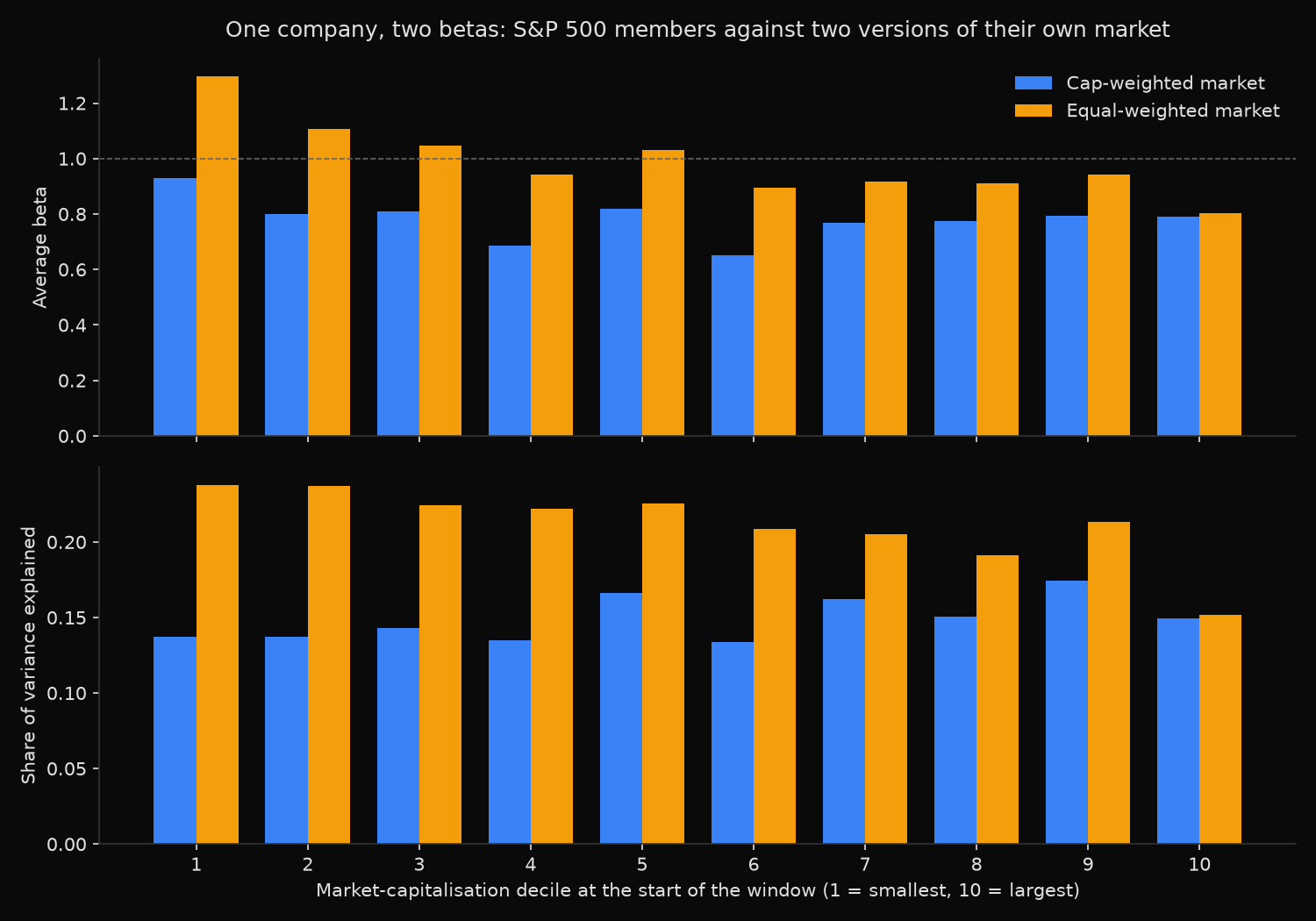
The average member has a beta of 0.783 to the cap-weighted market and 0.989 to the equal-weighted market. For 85.8 percent of companies the equal-weighted figure is the larger of the two, and the median gap is 0.238. Rank correlation between the two betas is 0.903, so the ordering of companies from low beta to high beta mostly survives; the levels do not.
Explanatory power moves the same way. The cap-weighted market accounts for 14.9 percent of the average member’s return variance and the equal-weighted market for 21.2 percent, with 82.2 percent of companies better explained by equal weight.
The decile table shows where the difference comes from. Among the smallest 47 members the average beta is 0.929 against cap weight and 1.295 against equal weight; in the largest decile the two nearly agree, at 0.791 and 0.802. Right at the top the ranking inverts: Microsoft measures 0.972 against the cap-weighted market and 0.663 against the equal-weighted one, Alphabet 0.989 and 0.651, Meta 1.325 and 0.788. A capitalisation index is largely the movement of its biggest constituents, so those constituents load on it heavily while a mid-sized company loads on it weakly. An equal-weighted market tracks the average stock, which is what a typical member happens to be.
Splitting the sample in half gives a rank correlation of 0.413 between the first-half gap and the second-half gap, and the average gap grew from 0.138 to 0.250, so the pattern is not a feature of one stretch of the window. A separate question, whether a beta measured in one window carries into the next, motivates a test of beta persistence built on two-year windows.
So what?
Record which benchmark a beta was measured against, because 0.783 and 0.989 are both correct answers to different questions. In a CAPM cost of equity, a difference of 0.206 in beta moves the risk premium term by about a fifth of whatever equity premium is assumed, wider than most judgment calls argued over in a valuation committee.
Hedging deserves the same care. Selling cap-weighted index futures against a portfolio of ordinary S&P 500 names sets the hedge ratio from a regression that explains 14.9 percent of the average name’s variance and leaves 28.7 percent annualised volatility behind. What remains is not only company-specific noise; it includes a systematic loading on the equal-weighted market that 82.2 percent of members carry. Before calling a long-short book market neutral, run the second regression against an equal-weighted market as well. It costs one extra line, and when the two betas disagree the position is holding a size and breadth exposure that the risk report is not showing.
Built with xfinlink — free financial data API for Python.