How Many Independent Bets Are There in the S&P 500? Principal Component Analysis in Python

August 29, 2026

What’s the question?

An S&P 500 fund holds five hundred companies, and a risk report on it lists five hundred line items. Neither number describes the risk being carried. The names do not move independently: most fall on the same days for the same reason, so the portfolio behaves like a much smaller set of positions bought repeatedly.

Principal component analysis puts a number on how much smaller. Take the correlation matrix of daily returns across the cross-section and extract its eigenvalues: each one is the variance sitting along an uncorrelated direction, and for N stocks they always sum to N. Independence puts one unit in each direction; total co-movement piles the whole N into the first, the direction usually called the market factor.

The spread of the eigenvalues collapses into one position count through their entropy:

N_eff = exp(-sum(p_i * ln p_i)),   p_i = lambda_i / N

N_eff lands on the same scale as the holding count: five hundred means five hundred genuine bets, thirty means thirty.

One estimation problem has to be settled first. A calendar year holds about 252 trading days against roughly 480 usable stocks, so the panel carries fewer observations than names, and sampling noise alone pushes the eigenvalues apart and drags N_eff down. The measure needs a yardstick for that noise.

The approach

The universe is the S&P 500 as it stood on 1 January of each year from 2015 to 2025, taken from point-in-time membership and carried by entity identifier rather than by symbol, so a reassigned ticker cannot splice two histories.

1. For each year, pull daily returns for that year’s members and keep the names that traded in every session, giving one clean panel per year.
2. Build the correlation matrix of those returns and take its eigenvalues.
3. Record the first component’s share of variance and the effective bet count from the entropy formula.
4. Repeat both measurements on a permuted copy of the panel: every stock keeps its own returns, but its dates are shuffled independently, destroying co-movement while leaving each name’s own distribution untouched.
5. Count the components whose eigenvalue exceeds the largest eigenvalue of the permuted panel, which are the directions sampling noise cannot account for.

The permutation is what makes the yearly figures readable: it says what the estimator returns for genuinely independent stocks over the same number of days, and that ceiling, not the holding count, is the yardstick. Every year carries one arithmetic check, since the eigenvalues must sum to the number of stocks.

Code

import numpy as np
import pandas as pd
import xfinlink as xfl

xfl.set_api_key("YOUR_API_KEY")  # free at https://xfinlink.com/signup

rng = np.random.default_rng(0)

def spectrum(matrix):
    corr = np.corrcoef(matrix, rowvar=False)
    return corr, np.sort(np.linalg.eigvalsh(corr))[::-1]

def effective_bets(eig, n):
    p = np.clip(eig / n, 1e-15, None)
    return float(np.exp(-(p * np.log(p)).sum()))

for year in range(2015, 2026):
    eids = sorted(xfl.index("sp500", as_of=f"{year}-01-01")["entity_id"])
    px = pd.concat([xfl.prices(entity_id=eids[i:i + 100], start=f"{year}-01-01",
                               end=f"{year}-12-31", fields=["return_daily"],
                               max_rows=200_000)
                    for i in range(0, len(eids), 100)], ignore_index=True)

    piv = px.pivot_table(index="date", columns="entity_id", values="return_daily")
    piv = piv[piv.notna().sum(axis=1) >= 100]
    A = piv[piv.columns[piv.notna().sum() == len(piv)]].values
    n = A.shape[1]

    corr, eig = spectrum(A)
    # each name keeps its own returns, its dates are shuffled: co-movement gone
    _, null = spectrum(np.column_stack([rng.permutation(A[:, j]) for j in range(n)]))

    print(year, n, round(eig[0] / n, 3), round(effective_bets(eig, n), 1),
          int((eig > null[0]).sum()), round(effective_bets(null, n), 1))

Full script with formatting and visualisation: how-many-independent-bets-sp500-pca-python.py

Output

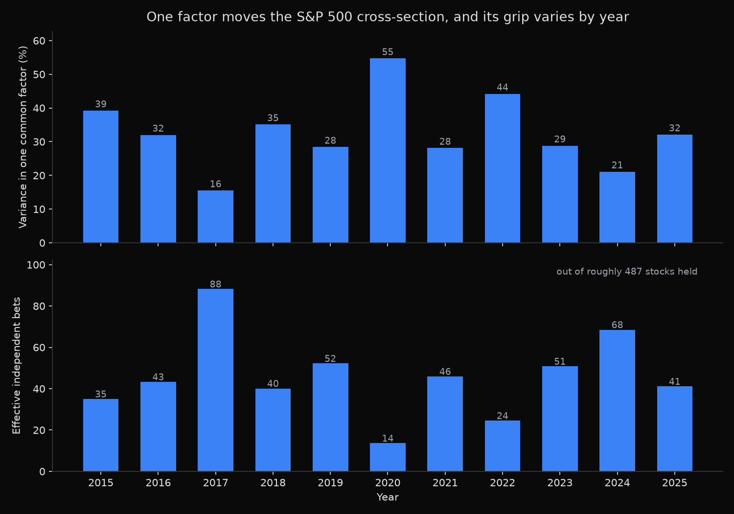
Point-in-time S&P 500 members, daily returns, one correlation matrix per year
Check: eigenvalues sum to the number of stocks in every year (largest gap 1.71e-13)

HOW MUCH OF THE CROSS-SECTION IS ONE COMMON FACTOR
  year  stocks  days     PC1    PC2  avg corr    bets  factors  port vol
  2015     474   252   39.2%   5.6%      0.37    35.0        6     15.8%
  2016     474   252   32.0%   8.1%      0.29    43.3        9     15.1%
  2017     482   251   15.5%   6.3%      0.13    88.2       11      7.4%
  2018     479   251   35.1%   7.0%      0.33    40.1        8     15.8%
  2019     486   252   28.4%   9.2%      0.25    52.2        9     12.9%
  2020     491   253   54.7%   7.7%      0.53    13.6        7     39.4%
  2021     493   252   28.1%   8.9%      0.25    45.9        9     13.9%
  2022     489   251   44.2%   6.2%      0.42    24.5        8     23.5%
  2023     495   250   28.8%   6.2%      0.27    50.8        9     14.5%
  2024     494   252   21.1%   7.7%      0.19    68.5       11     11.6%
  2025     487   250   32.1%   9.6%      0.29    41.1        8     17.6%

Widest dispersion : 2017  PC1 15.5%  88.2 bets from 482 stocks
Tightest year     : 2020  PC1 54.7%  13.6 bets from 491 stocks
Range of the effective bet count: 13.6 to 88.2   median 43.3

Permutation null (same stocks, same days, co-movement shuffled out)
  the estimator returns 192 to 195 bets when the names are genuinely independent
  components rising above that noise floor: 6 to 11 per year

PC1 share against the equal-weight portfolio's volatility: correlation 0.92 across 11 years
Volatility an equal-weight book removes versus the average single stock: 27% (2020) to 65% (2017)

What this tells us

The holding count and the bet count are never close. The index carried 474 to 495 stocks with a full year of trading, and the effective bet count ran from 13.6 to 88.2, median 43.3. The best year turned 482 positions into 88 bets; the worst turned 491 into fewer than 14.

Part of that gap is measurement rather than markets, which is what the permutation test is for. Shuffle each name’s dates and the same estimator returns 192 to 195 bets rather than the 480-odd stocks in the panel, because 250 days cannot resolve 490 independent directions. The ceiling worth comparing against is therefore about 193. The median year lands at 43.3 against it, under a quarter, and 2020 at 7%.

One direction dwarfs the rest in every year. Its share ranges from 15.5% in 2017 to 54.7% in 2020, while the second component never rises above 9.6%. The count of components clearing the noise floor is the steadiest number in the table: 6 in 2015, 11 in 2017 and 2024, 7 to 9 everywhere else. The number of distinguishable common drivers barely moves; what moves is how much variance the largest one takes.

The two things a portfolio cares about arrive together. The first component’s share tracks the annualised volatility of the equal-weight portfolio at a correlation of 0.92 across the eleven years. Holding all 482 names in 2017 removed 65% of the average single stock’s volatility; holding all 491 in 2020 removed 27%.

So what?

Size risk against the effective count rather than the position count. A book of 490 names supplying 14 bets carries the concentration of a fourteen-position portfolio, and a volatility target calibrated on the holding count is wrong by that factor exactly when it matters.

The 0.92 correlation is the part that bites. Diversification thins out in the years when volatility arrives, so a rule that adds exposure while realised risk is low buys more of a cross-section that has stopped behaving like one. Running the eigendecomposition on a trailing window turns that into a state variable visible before the drawdown.

The ceiling matters more for allocation than the level does. Between six and eleven directions clear the noise floor in any year, and adding the 501st US large-cap name does not create a twelfth. A mandate needing more independent bets than that has to source them outside this cross-section.

Built with xfinlink — free financial data API for Python. pip install -U xfinlink