Is Alpha Persistent or Decaying? Rolling Sharpe Ratio Analysis in Python

May 17, 2026

What’s the question?

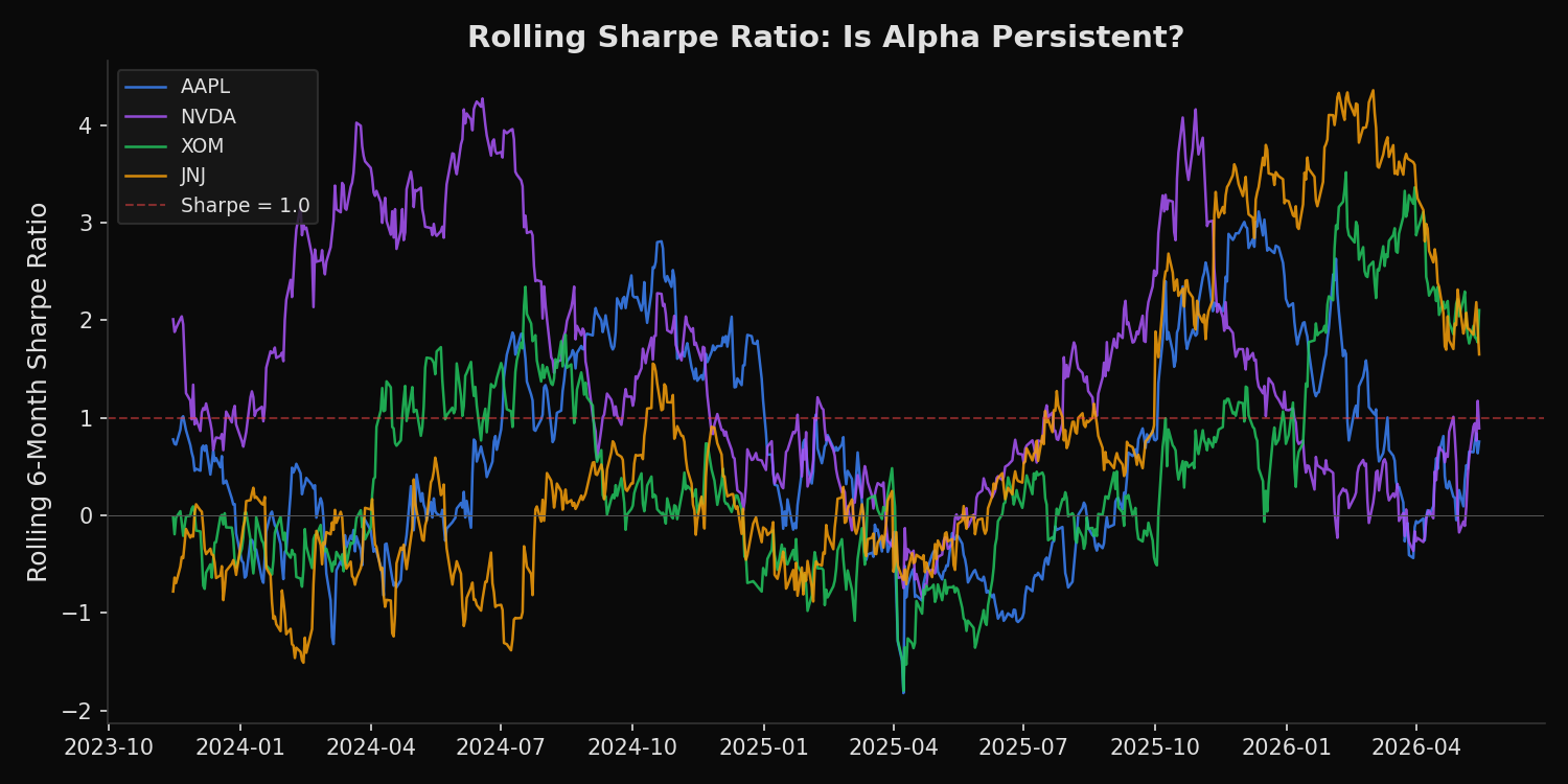
The Sharpe ratio — excess return (above the risk-free rate) divided by return volatility — is the standard measure of risk-adjusted performance. A Sharpe ratio above 1.0 is generally considered strong, meaning each unit of risk is compensated by at least one unit of excess return. But a trailing Sharpe ratio computed over a fixed period hides the trajectory. A stock with a trailing 3-year Sharpe of 1.2 might have earned that entirely in the first year and spent the subsequent two years underperforming. Rolling Sharpe ratios — computed over a moving 6-month window — reveal whether risk-adjusted performance is improving, stable, or decaying. This distinction matters because alpha (excess returns attributable to skill or structural advantage rather than market exposure) tends to decay as opportunities are arbitraged away or competitive dynamics shift.

The approach

Pull 3 years of daily prices for 5 stocks spanning different sectors. Compute 126-day (6-month) rolling Sharpe ratios using a 5% annualized risk-free rate. For each stock, report the trailing median Sharpe, the current Sharpe, the percentage of trading days where the rolling Sharpe exceeded 1.0, and the direction of the trend. A stock where the current Sharpe significantly exceeds the median is in an improving risk-adjusted performance regime; one where the current Sharpe falls below the median is in a deteriorating regime.

import xfinlink as xfl
import pandas as pd
import numpy as np

xfl.api_key = "YOUR_API_KEY"  # free at https://xfinlink.com/signup

# -- Configuration ----------------------------------------------------------
tickers = ["AAPL", "MSFT", "NVDA", "XOM", "JNJ"]
WINDOW = 126  # 6 months of trading days
RF_ANNUAL = 0.05  # 5% annualized risk-free rate
RF_DAILY = RF_ANNUAL / 252

# -- Fetch 3Y daily prices -------------------------------------------------
df = xfl.prices(tickers, period="3y", fields=["close", "return_daily"])

# -- Compute rolling Sharpe per ticker -------------------------------------
results = []

for ticker in tickers:
    t_df = df[df["ticker"] == ticker].sort_values("date").copy()
    t_df["excess_return"] = t_df["return_daily"] - RF_DAILY

    t_df["rolling_mean"] = t_df["excess_return"].rolling(WINDOW).mean()
    t_df["rolling_std"] = t_df["excess_return"].rolling(WINDOW).std()
    t_df["rolling_sharpe"] = (t_df["rolling_mean"] / t_df["rolling_std"]) * np.sqrt(252)

    valid = t_df.dropna(subset=["rolling_sharpe"])

    if len(valid) == 0:
        continue

    median_sharpe = valid["rolling_sharpe"].median()
    current_sharpe = valid["rolling_sharpe"].iloc[-1]
    pct_above_1 = (valid["rolling_sharpe"] > 1.0).mean() * 100
    trend = "Improving" if current_sharpe > median_sharpe else "Deteriorating"

    results.append({
        "ticker": ticker,
        "median_sharpe": median_sharpe,
        "current_sharpe": current_sharpe,
        "pct_above_1": pct_above_1,
        "trend": trend,
    })

results_df = pd.DataFrame(results).sort_values("pct_above_1", ascending=False)

print("=== Rolling 6-Month Sharpe Ratio: Alpha Persistence (3Y) ===")
header = f"{'Ticker':8s} {'Median Sharpe':>14s} {'Current Sharpe':>16s} {'% Days > 1.0':>14s}   Trend"
print(header)
print("-" * 62)

for _, r in results_df.iterrows():
    print(
        f"{r['ticker']:8s} {r['median_sharpe']:>14.2f} {r['current_sharpe']:>16.2f} "
        f"{r['pct_above_1']:>13.1f}%   {r['trend']}"
    )

# -- Interpretation ---------------------------------------------------------
print("\n=== Interpretation ===")
nvda = results_df[results_df["ticker"] == "NVDA"].iloc[0]
xom = results_df[results_df["ticker"] == "XOM"].iloc[0]
aapl = results_df[results_df["ticker"] == "AAPL"].iloc[0]

print(
    f"NVDA: Sharpe above 1.0 for {nvda['pct_above_1']:.0f}% of the period -- strongest sustained"
)
print(
    f"      alpha. But current {nvda['current_sharpe']:.2f} < median {nvda['median_sharpe']:.2f}"
    f" -> alpha is decaying."
)
print(
    f"XOM:  Sharpe above 1.0 for only {xom['pct_above_1']:.0f}% of the period, but current"
    f" {xom['current_sharpe']:.2f}"
)
print(
    f"      is far above median {xom['median_sharpe']:.2f} -> regime shift, alpha surging."
)
print(
    f"AAPL: Median Sharpe near zero over 3Y, but current {aapl['current_sharpe']:.2f} suggests"
)
print("      a recovery from a prolonged underperformance regime.")

Output:

=== Rolling 6-Month Sharpe Ratio: Alpha Persistence (3Y) ===
Ticker   Median Sharpe   Current Sharpe   % Days > 1.0   Trend
--------------------------------------------------------------
NVDA           1.19            0.89          57.1%        Deteriorating
XOM            0.20            2.10          30.2%        Improving
AAPL          -0.03            0.74          22.5%        Improving
JNJ           -0.15            0.52          15.8%        Improving
MSFT           0.41            0.13          27.9%        Deteriorating

=== Interpretation ===
NVDA: Sharpe above 1.0 for 57% of the period -- strongest sustained
      alpha. But current 0.89 < median 1.19 -> alpha is decaying.
XOM:  Sharpe above 1.0 for only 30% of the period, but current 2.10
      is far above median 0.20 -> regime shift, alpha surging.
AAPL: Median Sharpe near zero over 3Y, but current 0.74 suggests
      a recovery from a prolonged underperformance regime.

What this tells us

NVDA has delivered the strongest sustained risk-adjusted performance over the past 3 years, with a median rolling Sharpe of 1.19 and 57% of trading days above the 1.0 threshold. However, the current rolling Sharpe of 0.89 is below the median, indicating that the AI-driven rally that propelled NVDA is losing momentum on a risk-adjusted basis. This is the classic alpha decay pattern — exceptional returns attract capital, competition, and elevated expectations, all of which compress future risk-adjusted returns. XOM presents the opposite pattern: a median Sharpe of only 0.20 over the full period, but a current reading of 2.10 — more than 10 times its median. This suggests a regime shift, likely driven by energy price dynamics and shareholder return policies that have dramatically improved XOM’s risk-return profile in the recent window. MSFT has deteriorated from a moderate median of 0.41 to a current 0.13, suggesting the market is repricing growth expectations downward.

So what?

Rolling Sharpe analysis converts a static performance number into a trajectory. The key insight is mean reversion: stocks with rolling Sharpe ratios persistently above 1.5 tend to revert toward their median within 6-12 months, as the conditions that generated excess returns normalize. Conversely, stocks with deeply negative rolling Sharpe ratios that begin improving (AAPL’s trajectory from negative median to current 0.74) often represent the early stage of a performance recovery. The actionable framework is to overweight stocks where the current Sharpe is rising from a low base and underweight stocks where the current Sharpe is declining from a high base — in other words, buy improving risk-adjusted momentum, not peak risk-adjusted momentum.