What Growth Is Priced Into the S&P 500? Reverse DCF in Python

August 18, 2026

What’s the question?

A discounted cash flow model takes a forecast and returns a value. Every input is a judgement: how fast cash flow grows, for how long, and what rate discounts it back. Shift growth by two points and the answer moves by a third.

A reverse DCF turns the exercise around. The market has already set a price, so price becomes known and growth the unknown. Solving for the growth rate that makes model value equal market capitalisation produces one number: the growth an investor buying today is implicitly underwriting. Free cash flow here means cash from operations minus capital expenditure.

The inverted output can be falsified. "Priced at 34 times free cash flow" carries no obvious consequence, while "priced for 12.7 percent annual growth for a decade" is a claim that can be checked against the record. Does that implied rate carry information the multiple does not already contain, and does the growth the market prices resemble the growth companies have delivered?

The approach

The universe is the current S&P 500, addressed by permanent entity id. Financials and real estate leave the sample because free cash flow does not describe those businesses.

1. Sum free cash flow across the four most recent quarterly filings for a trailing twelve-month base, keeping only positive bases.
2. Take the median market capitalisation over the last 60 trading days, so one day’s price cannot drive the result.
3. Value one dollar of free cash flow: ten explicit years growing at g, then a perpetuity growing at 2.5 percent, discounted at 9 percent.
4. Solve for the g that sets model value equal to the observed price-to-free-cash-flow multiple, using Brent’s method over -40 percent to +60 percent. Multiples outside that range leave the sample.
5. Repeat at 8, 10 and 11 percent to separate what the price says from what the assumption says.
6. Compute delivered growth as the compound annual free cash flow rate from fiscal 2015 to fiscal 2025, matching the horizon.
7. Sort into price-to-free-cash-flow quintiles and set implied growth against delivered.

Model value rises monotonically in g, so the root is unique.

Code

import numpy as np
import pandas as pd
from scipy.optimize import brentq
import xfinlink as xfl

xfl.set_api_key("YOUR_API_KEY")  # free at https://xfinlink.com/signup

HORIZON, TERMINAL, RATE = 10, 0.025, 0.09
G_LO, G_HI = -0.40, 0.60

ids = xfl.index("sp500")["entity_id"].dropna().astype(int).tolist()
quarterly, annual, market = [], [], []
for i in range(0, len(ids), 50):
    b = ids[i:i + 50]
    quarterly.append(xfl.fundamentals(entity_id=b, period_type="quarterly", start="2025-01-01",
                                      fields=["free_cash_flow"], max_rows=50000))
    annual.append(xfl.fundamentals(entity_id=b, period_type="annual", start="2014-06-01",
                                   fields=["free_cash_flow", "fiscal_year"], max_rows=50000))
    market.append(xfl.prices(entity_id=b, start="2026-05-15",
                             fields=["close", "market_cap"], max_rows=200000))
q = pd.concat(quarterly, ignore_index=True)
a = pd.concat(annual, ignore_index=True)
p = pd.concat(market, ignore_index=True)

q = q.dropna(subset=["free_cash_flow"]).sort_values("period_end")
ttm = q.groupby("entity_id").tail(4).groupby("entity_id").agg(
    fcf_ttm=("free_cash_flow", "sum"), n_q=("free_cash_flow", "size"),
    last_q=("period_end", "max"))
ttm = ttm[(ttm["n_q"] == 4) & (ttm["last_q"] >= "2026-01-01")]

cap = p.dropna(subset=["market_cap"]).sort_values("date")
cap = cap.groupby("entity_id").tail(60).groupby("entity_id")["market_cap"].median() / 1e6

sector = a.sort_values("period_end").groupby("entity_id")["gics_sector"].last()
d = ttm.join(sector).join(cap.rename("mcap"))
d = d[~d["gics_sector"].isin({"Financials", "Real Estate"}) & d["gics_sector"].notna()]
d = d[(d["fcf_ttm"] > 0) & (d["mcap"] > 0)].copy()
d["pfcf"] = d["mcap"] / d["fcf_ttm"]


def model_multiple(g, r):
    """Value of $1 of current free cash flow, as a multiple, at growth g."""
    t = np.arange(1, HORIZON + 1)
    explicit = (((1 + g) ** t) / ((1 + r) ** t)).sum()
    terminal = (1 + g) ** HORIZON * (1 + TERMINAL) / ((r - TERMINAL) * (1 + r) ** HORIZON)
    return explicit + terminal


def implied_growth(multiple, r):
    f = lambda g: model_multiple(g, r) - multiple
    if f(G_LO) > 0 or f(G_HI) < 0:
        return np.nan
    return brentq(f, G_LO, G_HI, xtol=1e-9)


d["implied"] = d["pfcf"].apply(lambda m: implied_growth(m, RATE))
d["quintile"] = pd.qcut(d["pfcf"], 5, labels=False) + 1
print(d.groupby("quintile")[["pfcf", "implied"]].median())

Full script with formatting and visualisation: reverse-dcf-implied-growth-sp500-python.py

Output

sample: 323 S&P 500 members outside financials and real estate
model: 10 explicit years, 2.5% terminal growth, 9.0% discount rate

implied 10-year free-cash-flow growth, whole sample
  10th percentile    -3.7%
  median              7.3%
  90th percentile    20.0%

by price-to-free-cash-flow quintile
quintile      n   median P/FCF   implied growth   delivered growth
1 cheapest   65          10.0x           -3.7%               7.2%
2            64          15.7x            2.5%               7.3%
3            65          22.7x            7.3%               6.3%
4            64          31.3x           11.6%              10.7%
5 dearest    65          59.3x           20.1%              13.2%

discount rate sensitivity (median implied growth)
   8.0%      5.0%
   9.0%      7.3%
  10.0%      9.4%
  11.0%     11.4%
  1 point of discount rate moves implied growth by 2.12 points

implied vs delivered, 261 names with a full 10-year record
  median implied growth      6.9%
  median delivered growth    8.0%
  Spearman rank correlation   0.16
  priced above own delivered growth: 114 of 261 (44%)

What this tells us

The cheapest fifth trades at 10 times trailing free cash flow, and at a 9 percent discount rate that price implies free cash flow shrinking 3.7 percent a year for a decade. Those same companies grew it 7.2 percent a year over the previous ten. The dearest fifth trades at 59 times and needs 20.1 percent a year against 13.2 percent delivered.

Look at what the two middle columns have in common. Implied growth is a strictly increasing function of the multiple, so sorting on it reproduces the price-to-free-cash-flow order exactly and adds no cross-sectional information. It changes the unit: a multiple becomes a growth rate, and a growth rate is something an analyst can argue with.

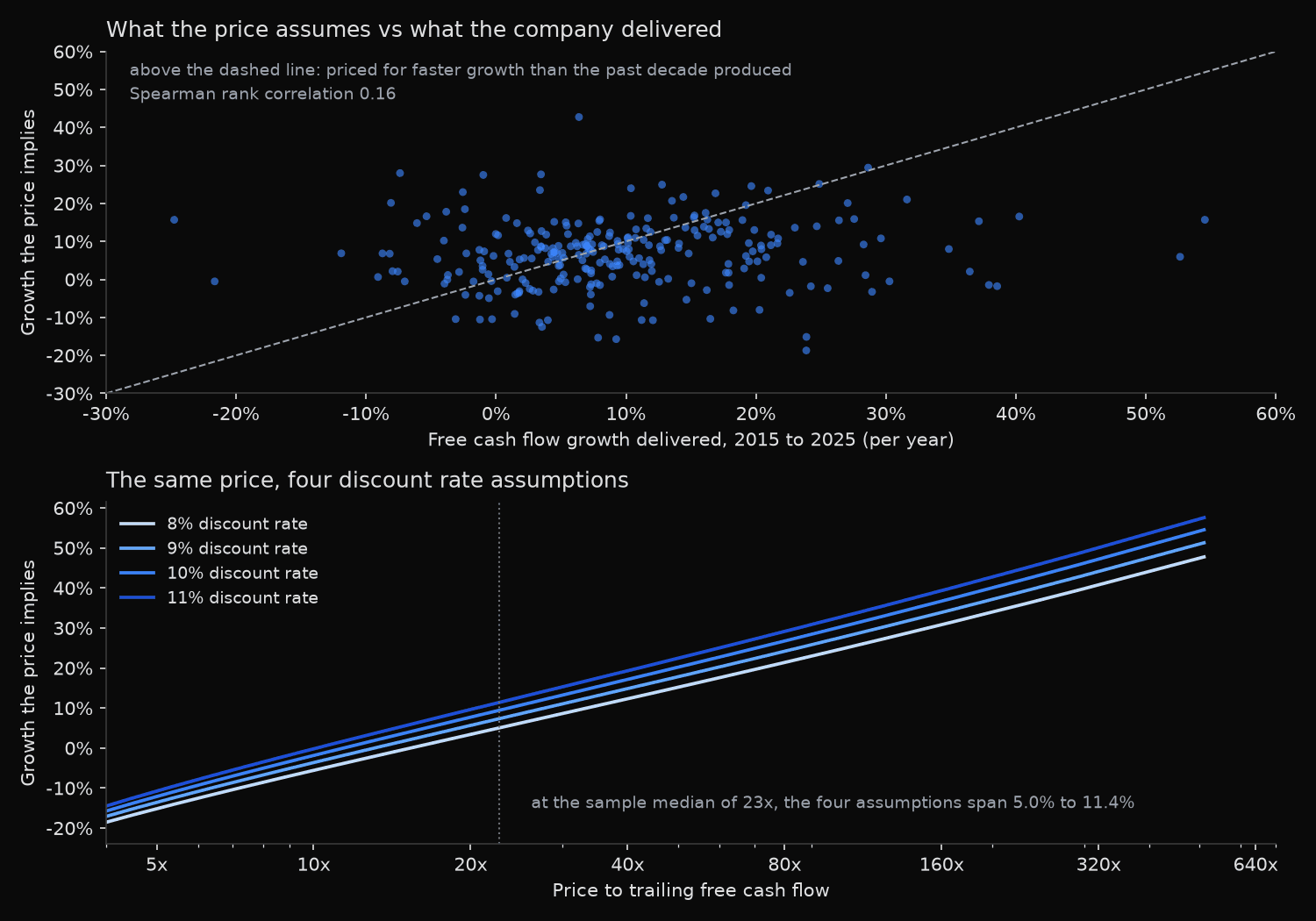
The lower panel shows where that translation gets fragile. Moving only the discount rate from 8 percent to 11 percent, with every price held fixed, lifts median implied growth from 5.0 percent to 11.4 percent: 2.12 points of growth per point of discount rate. Cost of equity is not observed; it is chosen. A colleague who prefers 10 percent to 9 percent reports a growth expectation more than two points higher on identical prices.

The comparison with delivered growth is the more uncomfortable result. Across the 261 names with a full ten-year record, the Spearman rank correlation between implied and delivered growth is 0.16, and only 114 carry an implied rate above their own delivered rate. Companies that compounded free cash flow quickly since 2015 are barely more likely to be priced for fast growth than companies that shrank. That is defensible rather than irrational: growth decays, and a decade of 30 percent compounding is a poor base case for the next.

So what?

Reverse DCF is a poor screen. Ranking on implied growth returns the same list as ranking on price to free cash flow, so anyone already sorting on the multiple gains nothing.

It works as a hypothesis to test. A cheapest-quintile price implying a 3.7 percent annual decline is a specific claim about revenue trend, contract renewals and competitive position. If that decline is absent from the operating data, the price needs explaining. The same logic runs in reverse for a name requiring 20.1 percent growth for ten years.

Publish the discount rate beside the growth number. Without the cost of equity a reader cannot separate the price signal from the analyst’s assumption.

One caveat governs where the method applies. Utilities contribute 6 names to a 323-name sample, because sustained capital spending leaves trailing free cash flow negative across that sector. Where capital expenditure is lumpy, normalise the base first, or the model charges a capex cycle to growth expectations.

Built with xfinlink — free financial data API for Python. pip install -U xfinlink