
What’s the question?
Operating leverage is the share of a company’s cost base that does not shrink when sales fall. Rent, depreciation on a factory, a salaried engineering team and a fibre network all cost roughly the same whether revenue rises 8 percent or drops 8 percent. A business built on those costs turns a small revenue move into a large profit move in both directions. A business whose costs are mostly the goods it buys and the hours it pays for behaves differently: profit tracks sales almost one for one.
The quantity that captures this is the degree of operating leverage, defined as the percentage change in operating income divided by the percentage change in revenue. A value near 1 means costs scale with sales. A value of 4 means a 10 percent revenue decline takes 40 percent of operating income with it.
Textbooks present that ratio for a single year, which is close to useless in practice because one year of noise can produce any number. Estimating it as a regression slope across a decade of filings gives something more stable, and it also produces a standard error, so the estimate can be judged rather than trusted.
The approach
The sample starts from the current S&P 500 roster. Financials and Real Estate are excluded, because operating income for a bank or a landlord is not built the same way as for a manufacturer and the two are not comparable on this measure.
- Pull eleven consecutive annual filings, FY2015 through FY2025, for revenue and operating income.
- Screen out any company where the profit base makes a percentage change meaningless: operating income must be positive in every one of the eleven years, and operating margin must be at least 3 percent in every year. A company whose operating income sits near zero or flips sign produces percentage changes in the hundreds or thousands, and a regression on those is arithmetic, not economics.
- For each survivor, compute ten annual percentage changes in revenue and ten in operating income, then regress the profit changes on the revenue changes. The slope is the estimated degree of operating leverage.
- Record the standard error and the p-value alongside the slope, and name companies only where the slope is distinguishable from zero at the 5 percent level. Ten observations is a small sample and many of the fits are not informative.
- Compute the annualised volatility of daily stock returns over 2015 to 2025 for each company, and compare it with the estimated slope.
166 companies clear every screen and hold a continuous daily price series under a single symbol across the whole window. Names without one drop from the sample.
Code
import numpy as np
import pandas as pd
import xfinlink as xfl
from scipy import stats

xfl.set_api_key("YOUR_API_KEY")  # free at https://xfinlink.com/signup

roster = xfl.index("sp500")
tickers = sorted(roster["ticker"].dropna().unique())

frames = [xfl.fundamentals(tickers[i:i + 100], period_type="annual",
                           start="2014-06-01", end="2026-06-30",
                           fields=["revenue", "operating_income"], max_rows=20000)
          for i in range(0, len(tickers), 100)]
fund = pd.concat(frames, ignore_index=True)
fund = fund[~fund["gics_sector"].isin(["Financials", "Real Estate"])]
fund = fund[fund["fiscal_year"].between(2015, 2025)]

rows = []
for ticker, g in fund.groupby("ticker"):
    g = g.sort_values("fiscal_year")
    if len(g) != 11 or g["operating_income"].min() <= 0:
        continue
    if (g["operating_income"] / g["revenue"]).min() < 0.03:
        continue

    d_rev = g["revenue"].pct_change().dropna().to_numpy() * 100
    d_opi = g["operating_income"].pct_change().dropna().to_numpy() * 100
    fit = stats.linregress(d_rev, d_opi)

    px = xfl.prices(ticker, start="2015-01-01", end="2025-12-31",
                    fields=["return_daily"])
    px = px[px["ticker"] == ticker].dropna(subset=["return_daily"])
    if len(px) < 2500:
        continue

    rows.append({"ticker": ticker, "slope": fit.slope, "r2": fit.rvalue ** 2,
                 "pval": fit.pvalue, "opinc_sd": d_opi.std(ddof=1),
                 "vol": px["return_daily"].std(ddof=1) * np.sqrt(252) * 100})

res = pd.DataFrame(rows).sort_values("slope", ascending=False)
sig = res[res["pval"] < 0.05]
print(f"{len(sig)} of {len(res)} slopes significant; "
      f"{(sig['slope'] > 1).sum()} of those above 1.0")
Full script with formatting and visualisation: operating-leverage-regression-python.py
Output
--------------------------------------------------------------------------
OPERATING LEVERAGE, FY2015-FY2025
slope = percent change in operating income per 1 percent change in revenue
--------------------------------------------------------------------------
sample: 166 current S&P 500 members outside Financials and Real Estate
        with 11 consecutive annual filings, operating income positive and
        operating margin at least 3% in every year
slopes distinguishable from zero at the 5% level: 85 of 166

HIGHEST SLOPES (5% significant only)
ticker sector                    slope    R2  op inc sd  stock vol
GLW    Information Technology     8.77  0.70     109.0%      30.0%
TEL    Information Technology     8.46  0.56     116.0%      27.0%
SBUX   Consumer Discretionary     6.79  0.68      74.7%      28.7%
ROST   Consumer Discretionary     5.50  0.91     102.4%      31.1%
FDX    Industrials                4.53  0.56      53.4%      31.9%
GWW    Industrials                4.20  0.74      23.3%      27.8%
CAT    Industrials                4.12  0.44      99.0%      30.0%
DG     Consumer Staples           3.79  0.83      23.3%      30.5%
NVDA   Information Technology     3.76  0.65     211.0%      48.7%
LH     Health Care                3.35  0.49      41.6%      26.1%

LOWEST SLOPES (5% significant only)
ticker sector                    slope    R2  op inc sd  stock vol
SNPS   Information Technology    -5.35  0.48      23.9%      33.0%
DVA    Health Care               -2.61  0.54      29.4%      31.7%
CPRT   Industrials                0.05  0.49      10.2%      26.5%
CI     Health Care                0.44  0.87      30.9%      30.4%
RSG    Industrials                0.74  0.63       8.5%      18.6%
AEE    Utilities                  0.79  0.45      11.5%      21.6%
GD     Industrials                0.82  0.42       8.8%      22.1%
HPQ    Information Technology     0.88  0.45      25.2%      34.4%
ROP    Information Technology     0.93  0.81      12.3%      22.6%
PH     Industrials                0.93  0.46      13.2%      30.9%

median slope, all 166 companies:  1.14
median slope, 85 significant:      1.65
significant slopes above 1.0: 72 of 85   below 0: 2 of 85

Spearman rank correlation with the slope
  volatility of annual operating-income growth: rho = +0.324, p = 2.0e-05
  annualised stock volatility:                  rho = +0.312, p = 4.3e-05

AVERAGES BY OPERATING-LEVERAGE QUARTILE
quartile       n  mean slope   op inc sd   stock vol
Q1 lowest     42       -0.51       24.7%       26.2%
Q2            41        0.86       21.1%       27.0%
Q3            41        1.52       19.6%       27.9%
Q4 highest    42        3.37       48.3%       31.5%

MEDIAN SLOPE BY SECTOR
Consumer Discretionary    10    1.80
Health Care               26    1.80
Communication Services     6    1.60
Information Technology    33    1.23
Industrials               44    1.23
Materials                  6    1.11
Consumer Staples          19    0.78
Energy                     4    0.74
Utilities                 18    0.36
What this tells us
Half the regressions carry no usable signal. Only 85 of 166 slopes are distinguishable from zero at the 5 percent level, which is the first honest result: ten annual observations, several of them from a pandemic year, will not identify an elasticity for a company whose revenue grows at a steady 6 percent every year. Companies with little variation in revenue growth have almost no information in the regressor, and their slopes should be discarded rather than ranked.
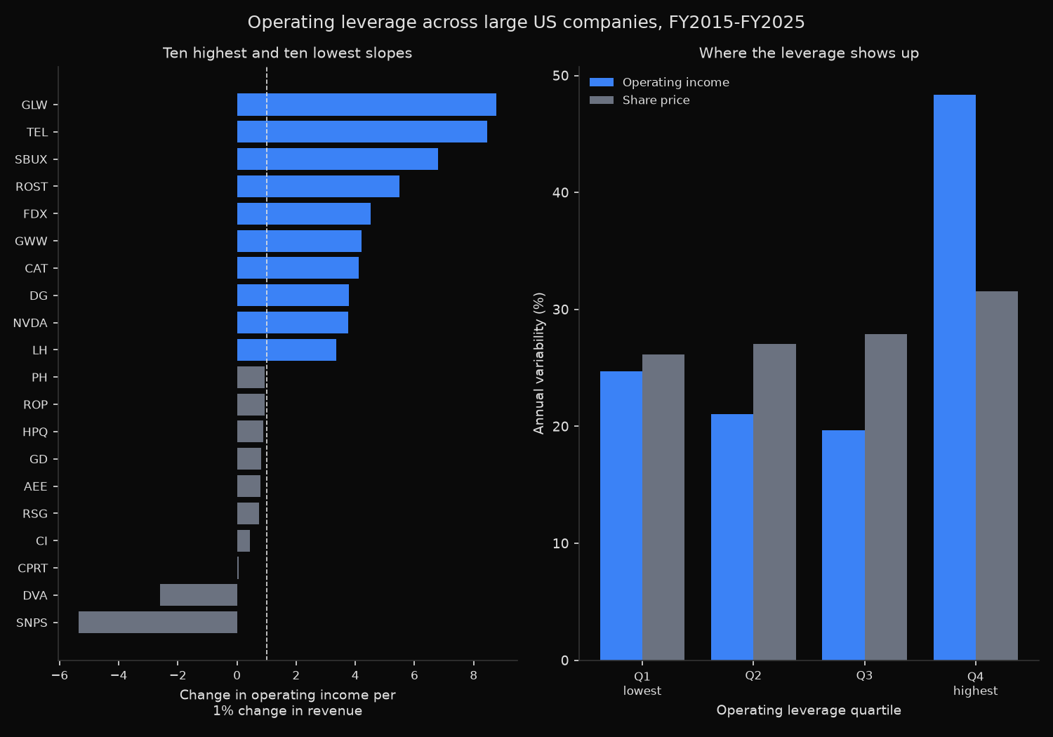
Where the slope is identified, it points one way. 72 of the 85 significant slopes exceed 1.0, and only 2 are negative. The median identified slope is 1.65, meaning a 1 percent revenue move typically carries operating income 1.65 percent. The extremes are large: at Corning’s 8.77 and TE Connectivity’s 8.46, a 10 percent revenue move implies an operating income move of roughly 88 and 85 percent, and both fits are reasonably tight, with R² of 0.70 and 0.56. Corning’s revenue rose from $9.1bn to $15.6bn across the window while operating income went from $1.3bn to a low of $509m and then to $2.3bn. That is what a heavy manufacturing base looks like when volume moves.
The sector ordering matches the underlying economics rather than any sector effect imposed on the data. Utilities sit last at a median slope of 0.36, which is the expected result for regulated businesses whose allowed return is set on a rate base rather than earned on volume. Consumer Discretionary and Health Care lead at 1.80.
The two negative significant slopes deserve naming, because a negative degree of operating leverage is a modelling artefact rather than a business property. Synopsys grew revenue every single year of the window, from $2.24bn to $7.05bn, so the regressor barely varies; the operating income path is dominated by acquisition and integration costs unrelated to that year’s sales growth. The regression fits a downward line through what is effectively a vertical scatter. Any slope estimated on a company with near-monotonic revenue growth should be read as an artefact of the fit.
The link to risk is where the result becomes interesting, and it is narrower than expected. Operating income variability roughly doubles across the quartiles, from 24.7 percent in the lowest-leverage group to 48.3 percent in the highest. Share price volatility rises over the same range by 5.3 percentage points, from 26.2 to 31.5 percent, a factor of 1.2. The rank correlation between slope and equity volatility is +0.312, real but modest. Operating leverage shows up forcefully in the earnings line and only faintly in the share price. A cross-sectional study of steady margins lines up margin variability, rather than leverage, against share-price volatility.
So what?
The practical use is in scenario work rather than screening. A demand forecast expressed in revenue terms translates into an earnings forecast through this slope, and using 1.0 by default understates the downside for most large companies. For Caterpillar at 4.12 or FedEx at 4.53, a 10 percent revenue shortfall is a 40 percent operating income shortfall, which is the difference between a disappointing year and a covenant conversation.
The gap between the earnings response and the price response is the part worth acting on. If a high-leverage company’s operating income swings twice as hard as a low-leverage one while its stock is only 20 percent more volatile, then equity volatility is a poor proxy for fundamental risk in the tail, precisely where it matters. Position sizing on trailing volatility alone will overweight names whose profits are one bad quarter of volume from halving.
Estimate the slope before relying on it, and check the p-value before quoting the number. Half of these regressions do not identify anything, and a confidently reported degree of operating leverage from a company with a decade of smooth revenue growth is a number with no content behind it.
Built with xfinlink — free financial data API for Python.