Does a Long Energy / Short Bonds Portfolio Capture Inflation Surprises? Factor Construction in Python

May 19, 2026

What’s the question?

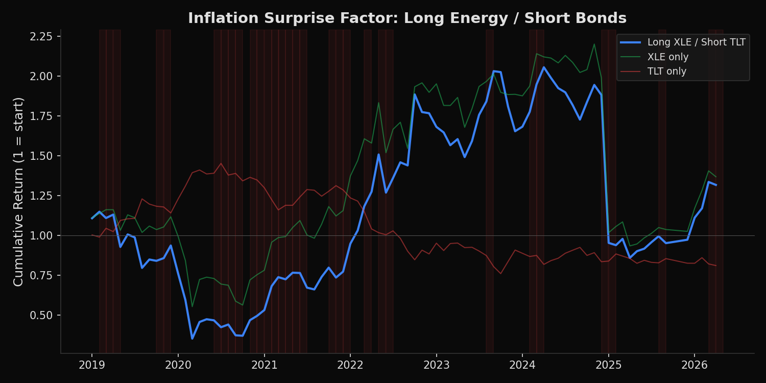
Inflation surprises — months where realized CPI exceeds the market’s prior expectation — should benefit assets that are positively correlated with inflation (energy, commodities) and harm assets that are negatively correlated (long-duration bonds). A zero-cost portfolio that is long energy (XLE) and short long-duration bonds (TLT) should therefore generate positive returns during inflationary surprises and negative returns during disinflationary surprises. If this portfolio reliably captures the inflation surprise premium, it functions as a tradeable inflation factor.

The approach

Construct CPI surprises by comparing actual month-over-month CPI changes to their 12-month trailing average (a naive expectation model). Classify months as HOT (surprise > 0.1%), COOL (surprise < -0.1%), or NEUTRAL. Compute returns of the long XLE / short TLT factor in each regime.

import xfinlink as xfl
import pandas as pd
import numpy as np
from fredapi import Fred

xfl.api_key = "YOUR_API_KEY"  # free at https://xfinlink.com/signup
fred = Fred(api_key=os.environ["FRED_API_KEY"])

# CPI from FRED
cpi = fred.get_series("CPIAUCSL", observation_start="2018-01-01")
cpi_mom = cpi.pct_change().dropna()
cpi_mom.index = cpi_mom.index.to_period("M")
cpi_mom = cpi_mom.rename("cpi_mom")
expected = cpi_mom.rolling(12).mean().rename("expected")
surprise = (cpi_mom - expected).rename("surprise")

# XLE, TLT monthly returns
tickers = ["XLE", "TLT"]
df = xfl.prices(tickers, start="2018-01-01", fields=["close"])
df["date"] = pd.to_datetime(df["date"])
monthly = df.groupby(["ticker", df["date"].dt.to_period("M")])["close"].last().unstack("ticker")
rets = monthly.pct_change().dropna()

# Factor = long XLE, short TLT
merged = pd.concat([rets, surprise], axis=1, join="inner").dropna()
merged["factor"] = merged["XLE"] - merged["TLT"]
merged["regime"] = pd.cut(merged["surprise"], bins=[-np.inf, -0.001, 0.001, np.inf],
                          labels=["COOL", "NEUTRAL", "HOT"])

for regime in ["HOT", "NEUTRAL", "COOL"]:
    sub = merged[merged["regime"] == regime]
    ann = sub["factor"].mean() * 12 * 100
    sharpe = sub["factor"].mean() / sub["factor"].std() * np.sqrt(12)
    print(f"{regime:8s} ({len(sub):2d} months): factor={ann:+.1f}%  Sharpe={sharpe:+.2f}")

Full script with formatting and visualisation: inflation-surprise-factor-python.py

Output:

Period: 2019-01 to 2026-04 (86 months)

HOT      (31 months):  factor=+26.0%  XLE=+15.0%  TLT=-11.0%  Sharpe=+0.55
NEUTRAL  (33 months):  factor=+28.1%  XLE=+30.2%  TLT=+2.1%  Sharpe=+0.78
COOL     (22 months):  factor=-23.0%  XLE=-17.7%  TLT=+5.3%  Sharpe=-0.49

Full sample:  ann_return=+14.3%  vol=43.3%  Sharpe=+0.33
Correlation with CPI surprise: +0.043

What this tells us

The factor behaves as theoretically expected: +26% annualized in HOT months, -23% in COOL months. The asymmetry is clean — energy outperforms bonds when inflation surprises to the upside, and bonds outperform energy when inflation disappoints. The NEUTRAL regime’s +28.1% return is driven by the secular energy rally of 2021-2025 rather than inflation dynamics. The full-sample Sharpe of 0.33 is modest, and the correlation with CPI surprises is only +0.04 — the factor captures the directional relationship but the signal-to-noise ratio is low because many other forces drive both XLE and TLT independently.

So what?

The long energy / short bonds factor does capture inflation surprises in the expected direction, but the low correlation (+0.04) and moderate Sharpe (0.33) mean it is not a standalone inflation hedge — it is one input in a multi-factor inflation portfolio. Combining it with TIPS breakeven rates, commodity futures, and inflation swap positions would improve the signal-to-noise ratio. The factor is most useful as a tactical overlay: increase allocation during periods when inflation expectations are rising and reduce it when disinflationary signals dominate.