
Log Returns vs Simple Returns: Which to Use
September 9, 2026
Use simple returns to combine holdings on a single date, and log returns to combine dates for a single holding. A simple return is the percentage change, P1/P0 - 1. A log return is the natural logarithm of the same ratio, ln(P1/P0). Each definition is additive along one axis only, and picking the wrong one produces errors that are large rather than cosmetic: Nvidia’s daily price returns from 2015 to 2024 add up to 675.9 percent, while its price actually rose 26,584.5 percent over that decade.
What Is the Difference Between a Log Return and a Simple Return?
Both measure the same move on different scales. A price going from 100 to 110 is a simple return of 0.10 and a log return of 0.0953. Falling from 110 back to 99 is a simple return of -0.10 and a log return of -0.1054.
Add the two simple returns and the answer is zero. An investor who held through both days has 99 dollars against the 100 they started with, so zero is wrong by a full percentage point. Add the two log returns and the answer is -0.0101, and exp(-0.0101) - 1 recovers -1.00 percent exactly. Multiplication in price space is addition in log space, and that single fact explains every practical difference between the two.
| Property | Simple return | Log return |
|---|---|---|
| Formula | P1/P0 - 1 | ln(P1/P0) |
| Adds across time | No | Yes |
| Averages across holdings | Yes | No |
| Range | -100 percent to unbounded | Unbounded either way, undefined at a total loss |
| Symmetry | +10 percent then -10 percent leaves a loss | +0.0953 then -0.0953 leaves nothing |
| Usual home | Portfolio weighting and attribution | Multi-period growth, volatility models |
When Should You Use Log Returns?
Whenever short periods are being combined into a longer one. Ten years of daily price returns for six large companies, all taken from split-adjusted closes over 2015 to 2024, show what the two aggregation rules do:
| Ticker | Daily returns added up | Compounded | exp(sum of log returns) |
|---|---|---|---|
| NVDA | 675.9% | 26,584.5% | 26,584.5% |
| AAPL | 262.1% | 816.2% | 816.2% |
| MSFT | 256.7% | 801.4% | 801.4% |
| XOM | 53.6% | 15.9% | 15.9% |
| JNJ | 48.8% | 38.4% | 38.4% |
| KO | 55.0% | 47.7% | 47.7% |
The last two columns agree to within a billionth of a percentage point, because they are the same calculation written twice. The first column is a different quantity that resembles a return and is not one.
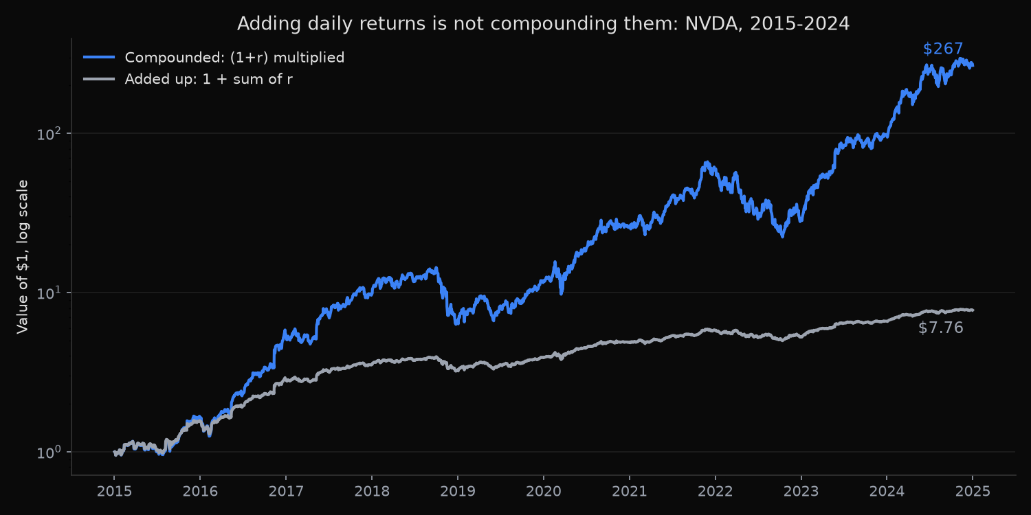
Exxon Mobil is the case worth pausing on. Its daily price returns sum to a cheerful +53.6 percent, and the share price over the same ten years rose 15.9 percent. The sum is not merely imprecise; on a volatile series it can point somewhere the position never went. A single log-space addition, exponentiated once at the end, is exact for any series and any horizon.
When Should You Use Simple Returns?
Whenever holdings are being combined into a portfolio on the same date. On 11 November 2016, Nvidia rose 29.81 percent and Coca-Cola rose 0.22 percent. Half of each, rebalanced that morning, returned 15.01 percent, which is the plain average of the two percentages. Averaging the two log returns and converting back gives 14.06 percent, which no portfolio earned.
Most days the gap is invisible. Across the same decade the mean absolute difference between the two methods for that pair is 0.012 percentage points a day, and it never cancels, because the log-averaged version is always the lower of the two. Compounding is what makes it matter: an equal-weight Nvidia and Coca-Cola position rebalanced daily grew 2,550.7 percent in price terms over the ten years, against 1,885.6 percent built from averaged logs. A hundredth of a point a day, repeated 2,515 times, costs a quarter of the terminal wealth.
The rule is mechanical. Weights multiply prices, not logarithms of prices, so cross-sectional arithmetic belongs in simple space. Convert to logs afterwards if the portfolio series then has to be chained through time.
Why Is the Average Log Return Smaller Than the Average Simple Return?
Because the logarithm is concave, the mean log return sits below the mean simple return by approximately half the variance. This is the variance drag, and it is the reason a volatile asset needs a higher average return to reach the same compound growth as a quiet one.
| Ticker | Annualised volatility | Mean simple return x 252 | Mean log return x 252 | Gap | Half the variance |
|---|---|---|---|---|---|
| NVDA | 48.6% | 67.7% | 56.0% | 11.7 | 11.8 |
| AAPL | 28.5% | 26.3% | 22.2% | 4.1 | 4.1 |
| MSFT | 27.2% | 25.7% | 22.0% | 3.7 | 3.7 |
| XOM | 27.9% | 5.4% | 1.5% | 3.9 | 3.9 |
| JNJ | 18.1% | 4.9% | 3.3% | 1.6 | 1.6 |
| KO | 17.8% | 5.5% | 3.9% | 1.6 | 1.6 |
The last two columns match to within 0.07 percentage points on every name, which is the identity holding in live data rather than in a textbook. Nvidia pays 11.7 points a year for its volatility; Coca-Cola pays 1.6.
The practical consequence is a reporting one. Multiplying an average daily return by 252 does not give the growth rate a position delivered, in either direction. Nvidia’s compound annual price growth over the decade was 75.0 percent, its annualised mean simple return 67.7 percent, and its annualised mean log return 56.0 percent, and only the first describes what the position did. Quote a growth rate as exp(252 x mean log return) - 1, or compute it from the first and last price and skip the averaging.
What Does the Data Have to Get Right?
Both definitions inherit whatever the price series gets wrong, and there is one failure that dwarfs the rest. A raw close series steps down on split dates, so a 4-for-1 split reads as a 75 percent loss in simple space and as -1.39 in log space, and no arithmetic downstream can repair it. The series has to be split-adjusted before either formula runs. In xfinlink, adj_close is backward-adjusted for splits and continuous across them, while close stays as traded; the mechanics are set out in split adjustment explained, and the why prices differ between sources guide covers the adjustment choices that make two vendors disagree on the same day.
One call returns the series for the whole basket, and both return definitions come from the same three lines:
import numpy as np
import pandas as pd
import xfinlink as xfl

xfl.set_api_key("YOUR_API_KEY")  # free at https://xfinlink.com/signup

tickers = ["NVDA", "AAPL", "MSFT", "XOM", "JNJ", "KO"]
px = xfl.prices(tickers, start="2015-01-01", end="2024-12-31", fields=["adj_close"])

for t in tickers:
    s = px[px["ticker"] == t].sort_values("date")["adj_close"]
    simple = s.pct_change().dropna()
    log = np.log1p(simple)
    print(t, round(100 * simple.sum(), 1),
          round(100 * ((1 + simple).prod() - 1), 1),
          round(100 * (np.expm1(log.sum())), 1))
NVDA 675.9 26584.5 26584.5
AAPL 262.1 816.2 816.2
MSFT 256.7 801.4 801.4
XOM 53.6 15.9 15.9
JNJ 48.8 38.4 38.4
KO 55.0 47.7 47.7adj_close carries no dividend component, so the figures above are price returns; the same arithmetic applies unchanged to any total-return series you build. Field definitions are in the docs. A free key covers a rolling twelve months of history at one ticker per call, and full history back to 1996 comes with the paid plans on the pricing page.
FAQ
Are the two close enough to ignore on daily data? For ordinary sessions, yes: below about one percent a day they differ by less than a hundredth of a percentage point, because the gap grows with the square of the move. On Nvidia’s best day in the sample the simple return is 29.81 percent and the log return 26.09 percent, so the equivalence stops holding exactly where the interesting days are.
Which one should a volatility estimate use? Log returns are the usual input, since option pricing and most volatility models assume the logarithm is the normally distributed quantity. At daily frequency the two standard deviations differ little. Consistency matters more than the choice, so record which one an estimate used.
Can log returns handle a total loss? No. A price falling to zero gives a log return of negative infinity, so bankruptcies, liquidations and any series with a zero or missing price need handling before the logarithm runs. Simple returns are bounded below at -100 percent and survive the same event.
Built with xfinlink — free financial data API for Python. pip install -U xfinlink
pip install -U xfinlink