
How Many Days of Data Does a Volatility Estimate Need? Range-Based Estimators in Python
August 4, 2026
What’s the question?
Volatility feeds almost every risk calculation, and it is never observed directly. It has to be estimated from past prices, so every estimate carries sampling error. The standard recipe squares daily log returns and averages them: one number per day, and everything the price did in between is discarded.
Picture a fund that opens at 100, trades up to 104, sinks to 97, and closes at 100. The close-to-close return is zero. The day was violent and the estimator records nothing.
Four estimators read the rest of the bar. Parkinson (1980) uses the high-low range, whose expected square for a driftless random walk is 4·ln(2) times the variance. Garman-Klass (1980) folds in the open and the close. Rogers-Satchell (1991) rearranges the terms so that a price with drift does not bias the answer. Yang-Zhang (2000) adds a term for the gap between yesterday’s close and today’s open, which the other three cannot see.
The textbook claim: a day’s high-low range carries roughly five times the information about volatility that the close does. That figure comes from a model with fixed volatility and a continuously watched price path. Real bars honour neither condition.
The approach
True volatility is unknown and it moves, so estimator error cannot be measured against it. A split sample gets around that.
- Eight liquid ETFs over ten years, 2016-08-01 to 2026-08-03, spanning US large, small and mega caps (SPY, IWM, DIA), markets outside the US (EFA, EEM), long Treasuries (TLT) and two sectors (XLK, XLF). Each fund has a bar for every session in the window.
- Convert each bar to logs relative to the prior close, after multiplying the open, high and low by adj_close/close so that a share split registers as a change of units rather than an overnight move.
- Cut each series into consecutive blocks of 22 trading days, sending odd-numbered days into one half and even-numbered days into the other. Both halves hold 11 days from the same month of market conditions.
- Compute all five estimators on each half and take the difference of their logs. The two halves measure the same volatility, so what separates them is sampling noise.
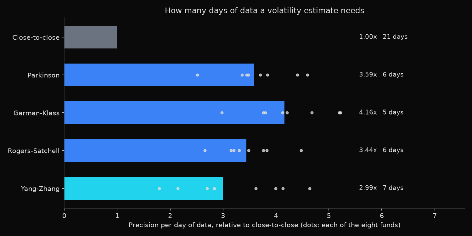
- Precision is the variance of the close-to-close differences divided by the variance of the estimator’s own, pooled across 912 block pairs.
A precision of 4 means one day of that estimator carries as much information as four days of closes.
Code
import numpy as np
import pandas as pd
import xfinlink as xfl

xfl.set_api_key("YOUR_API_KEY")  # free at https://xfinlink.com/signup

TICKERS = ["SPY", "IWM", "DIA", "EFA", "EEM", "TLT", "XLK", "XLF"]
NAMES = ["close_to_close", "parkinson", "garman_klass", "rogers_satchell", "yang_zhang"]
NHALF = 11

px = xfl.prices(TICKERS, start="2016-08-01", end="2026-08-03",
                fields=["open", "high", "low", "close", "adj_close"])

def estimators(o, h, l, c):
    """Daily variance estimates. Inputs are logs relative to the prior close."""
    n = len(c)
    hl, co, u, d = h - l, c - o, h - o, l - o
    rs = np.mean(u * (u - co) + d * (d - co))
    k = 0.34 / (1.34 + (n + 1) / (n - 1))
    return {
        "close_to_close": np.mean(c ** 2),
        "parkinson": np.mean(hl ** 2) / (4 * np.log(2)),
        "garman_klass": np.mean(0.5 * hl ** 2 - (2 * np.log(2) - 1) * co ** 2),
        "rogers_satchell": rs,
        "yang_zhang": np.var(o, ddof=1) + k * np.var(co, ddof=1) + (1 - k) * rs,
    }

gaps = []
for tk in TICKERS:
    t = px[px["ticker"] == tk].sort_values("date")
    f = t["adj_close"] / t["close"]      # split factor: puts o/h/l on the adj_close basis
    prev = t["adj_close"].shift(1)
    m = pd.DataFrame({"o": np.log(t["open"] * f / prev), "h": np.log(t["high"] * f / prev),
                      "l": np.log(t["low"] * f / prev), "c": np.log(t["adj_close"] / prev)
                      }).dropna().to_numpy()
    for b in range(len(m) // (2 * NHALF)):
        blk = m[b * 2 * NHALF:(b + 1) * 2 * NHALF]
        A, B = estimators(*blk[0::2].T), estimators(*blk[1::2].T)
        gaps.append({k: np.log(A[k]) - np.log(B[k]) for k in NAMES})

G = pd.DataFrame(gaps)
base = G["close_to_close"].var(ddof=1)
for k in NAMES:
    print(f"{k:>16} precision={base / G[k].var(ddof=1):.2f}")
Full script with formatting and visualisation: range-based-volatility-estimators-python.py
Output
Annualised volatility by estimator, 20,120 daily bars, 2016-08-01 to 2026-08-03

        Close-to-close  Parkinson  Garman-Klass  Rogers-Satchell  Yang-Zhang
ticker
SPY              18.07      13.78         13.87            14.03       18.18
IWM              23.14      18.62         18.84            19.03       23.76
DIA              17.64      12.92         12.92            13.05       17.36
EFA              17.28      10.13         10.06            10.12       17.40
EEM              20.98      11.84         11.85            12.00       21.10
TLT              14.84      10.09         10.00             9.91       14.80
XLK              24.96      18.60         18.37            18.39       24.40
XLF              22.19      16.62         16.85            17.15       22.88

Sampling noise, 912 odd/even half-block pairs of 11 days each

       estimator  ann vol %  noise sd  precision  days for 21
  Close-to-close      20.13     0.740       1.00         21.0
       Parkinson      14.44     0.391       3.59          5.9
    Garman-Klass      14.47     0.363       4.16          5.0
 Rogers-Satchell      14.60     0.399       3.44          6.1
      Yang-Zhang      20.28     0.427       2.99          7.0

precision range across the eight funds
        Parkinson: 2.52 to 4.60
     Garman-Klass: 2.98 to 5.22
  Rogers-Satchell: 2.66 to 4.48
       Yang-Zhang: 1.80 to 4.64
What this tells us
The high and low are worth a great deal. Garman-Klass extracts 4.16 times as much precision per day as close-to-close, so five trading days of open-high-low-close bars pin down volatility as tightly as 21 days of closing prices. Parkinson reaches 3.59 and Rogers-Satchell 3.44, both using less of the bar.
The levels tell a second story. Across the pooled sample, Parkinson, Garman-Klass and Rogers-Satchell read about 28 percent below close-to-close in volatility terms, which is roughly half the variance, though the size of that gap varies from fund to fund. They see the trading session and nothing outside it. Yang-Zhang, the one estimator carrying a gap term, lands within 3.2 percent of close-to-close on all eight funds while still delivering 2.99 times the precision. Same quantity, one third of the data.
Measured precision sits below the published figures of 5.2 for Parkinson and 7.4 for Garman-Klass, for the two reasons named earlier: volatility moves inside a 22-day block, adding noise that every estimator inherits and dragging the ratios toward one, and discrete trading clips the true high and low. These figures are a floor.
Yang-Zhang’s precision varies most across funds, from 1.80 on EEM to 4.64 on XLK. Its gap term is an ordinary variance of 11 numbers and inherits close-to-close’s inefficiency, so the more of the daily move that lands before the opening bell, the less Yang-Zhang gains. EEM and EFA track markets that trade while the US is shut, which is why their session-only estimates sit furthest below close-to-close: 10.13 against 17.28 for EFA.
So what?
Pick the estimator to match the risk being measured, then shorten the window.
For total daily volatility, the input to position sizing and risk limits, Yang-Zhang is the choice. Seven trading days of it match 21 days of closes, and a rolling window lags a change in volatility by roughly half its length, so the shorter window turns about a week sooner at the same noise level. For session risk, where execution and stop placement live, Garman-Klass does the same job in five days.
Levels must not be mixed. Replacing a close-to-close volatility with a Parkinson volatility looks like a 28 percent fall in risk that has not happened, and an option priced off that number will be too cheap. Any cross-desk or cross-vendor comparison has to establish which estimator produced each figure first.
Before committing, measure how much of a fund’s move lands outside the session. Where that share is large, as it is for funds tracking foreign markets, the gain is real but smaller than the headline.
Built with xfinlink — free financial data API for Python. pip install -U xfinlink
pip install -U xfinlink