Can Risk Parity Tame Commodity Volatility? Portfolio Optimization in Python

June 18, 2026

What's the question?

An equal-weight commodity basket can look diversified by ticker count while still being dominated by the most volatile instruments. Natural gas and oil can drive total risk even when their capital weights are the same as gold or agriculture.

Risk parity is a portfolio construction method that attempts to balance risk contributions rather than dollar weights. A simple version uses inverse volatility: lower-volatility assets receive larger weights, and higher-volatility assets receive smaller weights.

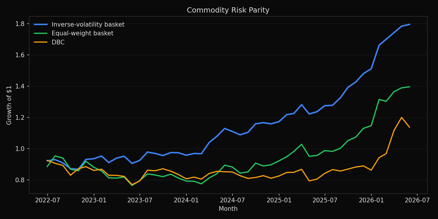
The question is whether inverse-volatility weighting improves the return, volatility, and drawdown profile of a commodity basket.

The approach

The portfolio universe is GLD, SLV, USO, UNG, DBA, and DBB. DBC is used as a broad commodity benchmark. Built from SEC EDGAR public filings and market data, the backtest uses five years of daily returns converted into complete monthly returns.

1. Pull five years of daily returns
2. Compound daily returns into monthly returns
3. Estimate trailing 12-month volatility for each ETF
4. Allocate weights in inverse proportion to volatility
5. Compare inverse-volatility weights with equal weight and DBC

Weights are shifted by one month because the trailing volatility estimate must be known before the next month's return is earned.

Code

import xfinlink as xfl
import pandas as pd
import numpy as np

xfl.set_api_key("YOUR_API_KEY")  # free at https://xfinlink.com/signup

tickers = ["GLD", "SLV", "USO", "UNG", "DBA", "DBB"]
prices = xfl.prices(tickers + ["DBC"], period="5y", fields=["return_daily"])
daily = prices.pivot_table(index="date", columns="ticker", values="return_daily").dropna()

monthly = (1 + daily).resample("ME").prod() - 1
rolling_vol = monthly[tickers].rolling(12).std().shift(1)

inverse_vol = 1 / rolling_vol
weights = inverse_vol.div(inverse_vol.sum(axis=1), axis=0).dropna()

risk_parity = (monthly.loc[weights.index, tickers] * weights).sum(axis=1)
equal_weight = monthly.loc[weights.index, tickers].mean(axis=1)

print((1 + risk_parity).prod(), (1 + equal_weight).prod())

Full script with formatting and visualisation: commodity-risk-parity-python.py

Output

=== Commodity Risk Parity Backtest ===
Universe: GLD, SLV, USO, UNG, DBA, DBB
Sample: 2022-06-30 to 2026-05-31 (48 monthly observations)
Weight rule: inverse trailing 12-month volatility, rebalanced monthly

Portfolio comparison:
Inverse-vol basket   return=+15.7%  vol=11.7%  sharpe= 1.34  max_drawdown= -6.7%  positive_months=68.8%
Equal-weight basket  return= +8.7%  vol=16.0%  sharpe= 0.54  max_drawdown=-19.8%  positive_months=56.2%
DBC benchmark        return= +3.3%  vol=15.2%  sharpe= 0.22  max_drawdown=-16.7%  positive_months=52.1%

Latest inverse-volatility weights:
DBB  weight=33.8%
DBA  weight=30.5%
GLD  weight=15.4%
SLV  weight= 8.3%
USO  weight= 6.0%
UNG  weight= 5.9%

What this tells us

Inverse-volatility weighting materially improved the commodity basket in this sample. The inverse-volatility basket returned 15.7% annualized, compared with 8.7% for equal weight and 3.3% for DBC. It also reduced volatility to 11.7%.

The drawdown improvement is the most important result. The inverse-volatility basket had a maximum drawdown of -6.7%, while the equal-weight basket fell -19.8% and DBC fell -16.7%. The strategy worked because it prevented the highest-volatility exposures from dominating portfolio risk.

The latest weights show the mechanism. DBB and DBA receive the largest allocations, while USO and UNG receive the smallest. This is not a view that energy is unattractive. It is a risk-control rule that acknowledges the larger loss distribution in those instruments.

So what?

Commodity diversification should be measured by risk, not by the number of tickers. Equal weight gives the same capital allocation to instruments with very different volatility and drawdown profiles. That can turn a diversified basket into an energy-driven portfolio.

Inverse-volatility weighting is a practical baseline. It is simple, transparent, and easy to rebalance. More advanced risk parity models can include correlations and target equal risk contribution, but the first-order improvement comes from reducing exposure to the most volatile commodities before they dominate the portfolio.

Built with xfinlink — free financial data API for Python. pip install xfinlink