How Many Calendar Anomalies Survive Multiple Testing? Bootstrap Reality Check in Python

September 14, 2026

What’s the question?

A calendar anomaly usually arrives wearing a single number. Hold the S&P 500 only on Thursdays in April, the claim goes, and those days average a quarter of a percent while ordinary days average a small fraction of that; the t-statistic clears 2, so the pattern is real.

The arithmetic is correct and the inference is not, because the rule was never fixed before the data were examined. It won a search. A t-test judges one hypothesis chosen in advance, and the largest of sixty noisy quantities runs high even when all sixty are noise.

The question is where the hurdle really sits. If a person tests every month-by-weekday rule on an index fund and reports the best, what t-statistic does that search produce on chance alone?

The approach

Daily returns on three index funds carry the test: SPY for the S&P 500, QQQ for the Nasdaq 100, IWM for the Russell 2000. The window runs from 1 January 1996 to 31 December 2024, each fund entering on its first trading day. The candidate family is every pairing of calendar month with weekday, so 12 months times 5 weekdays produces 60 rules, each holding the fund only on days carrying both labels. That family matches the shape of rule people actually mine.

1. Compute a Welch t-statistic for every rule, comparing its days against all other days, and record the winner.
2. Resample the returns 2,000 times with a circular block bootstrap of length 10, holding the calendar labels fixed so returns and dates shuffle apart. Ten-day blocks preserve volatility clustering and autocorrelation inside each resampled series.
3. Run the same 60-rule search on every resampled series and keep its winner. Those 2,000 winners form the distribution of the best result this size of search returns when no rule is real.
4. Read the share of resampled searches beating the real winner as the snooping-adjusted p-value, and the 95th percentile as the honest 5% hurdle.

A procedure that always answers no would be worthless, so a further step plants a known effect on every September Tuesday in SPY, at two sizes, and repeats the search.

Code

import numpy as np
import pandas as pd
import xfinlink as xfl
from scipy import stats

xfl.set_api_key("YOUR_API_KEY")  # free at https://xfinlink.com/signup

px = xfl.prices("SPY", start="1996-01-01", end="2024-12-31", fields=["return_daily"])
px = px.dropna(subset=["return_daily"]).sort_values("date").reset_index(drop=True)
dates = pd.DatetimeIndex(px["date"])
r = px["return_daily"].to_numpy()

M = np.array([(dates.month.values == m) & (dates.dayofweek.values == w)
              for m in range(1, 13) for w in range(5)], dtype=float)

def welch_t(r, M):
    n = len(r)
    n_in = M.sum(1)
    n_out = n - n_in
    s1, s2 = M @ r, M @ (r ** 2)
    m_in, m_out = s1 / n_in, (r.sum() - s1) / n_out
    v_in = (s2 - n_in * m_in ** 2) / (n_in - 1)
    v_out = (((r ** 2).sum() - s2) - n_out * m_out ** 2) / (n_out - 1)
    return (m_in - m_out) / np.sqrt(v_in / n_in + v_out / n_out)

t_best = welch_t(r, M).max()

rng = np.random.default_rng(7)
n, n_blocks = len(r), int(np.ceil(len(r) / 10))
boot = np.empty(2000)
for b in range(2000):
    idx = (rng.integers(0, n, n_blocks)[:, None] + np.arange(10)).ravel()[:n] % n
    boot[b] = welch_t(r[idx], M).max()

print("best t", round(float(t_best), 2))
print("p, one test", round(float(2 * (1 - stats.norm.cdf(t_best))), 4))
print("p, best of 60", float((boot >= t_best).mean()))
print("5% hurdle", round(float(np.percentile(boot, 95)), 2))

Full script with formatting and visualisation: calendar-anomaly-multiple-testing-bootstrap-python.py

Output

Best-of-60 calendar rules | month x weekday | 1996-01-01 to 2024-12-31
Bootstrap: 2,000 circular block draws, block length 10

SPY (S&P 500) 1996-01-02 to 2024-12-31  7,300 trading days, smallest rule cell 88
  best rule           Apr-Thu  (124 days, mean +0.252% per day)
  t-statistic         2.28
  p-value, one test   0.0225
  p-value, best of 60 0.5105
  5% hurdle for t     3.14  (single-test hurdle 1.96)
  rules with |t|>1.96 2  (3.0 expected by chance)

QQQ (Nasdaq 100) 1999-03-11 to 2024-12-31  4,907 trading days, smallest rule cell 55
  best rule           Oct-Thu  (88 days, mean +0.517% per day)
  t-statistic         2.32
  p-value, one test   0.0203
  p-value, best of 60 0.4840
  5% hurdle for t     3.11  (single-test hurdle 1.96)
  rules with |t|>1.96 3  (3.0 expected by chance)

IWM (Russell 2000) 2000-05-30 to 2024-12-31  6,187 trading days, smallest rule cell 73
  best rule           May-Mon  (82 days, mean +0.316% per day)
  t-statistic         1.58
  p-value, one test   0.1152
  p-value, best of 60 0.9875
  5% hurdle for t     3.20  (single-test hurdle 1.96)
  rules with |t|>1.96 1  (3.0 expected by chance)

Power check: a known effect added to every September Tuesday in SPY
  +0.25% per day planted -> winner Apr-Thu, t 2.24, p-value best of 60 0.5770
  +0.50% per day planted -> winner Sep-Tue, t 3.42, p-value best of 60 0.0180

What this tells us

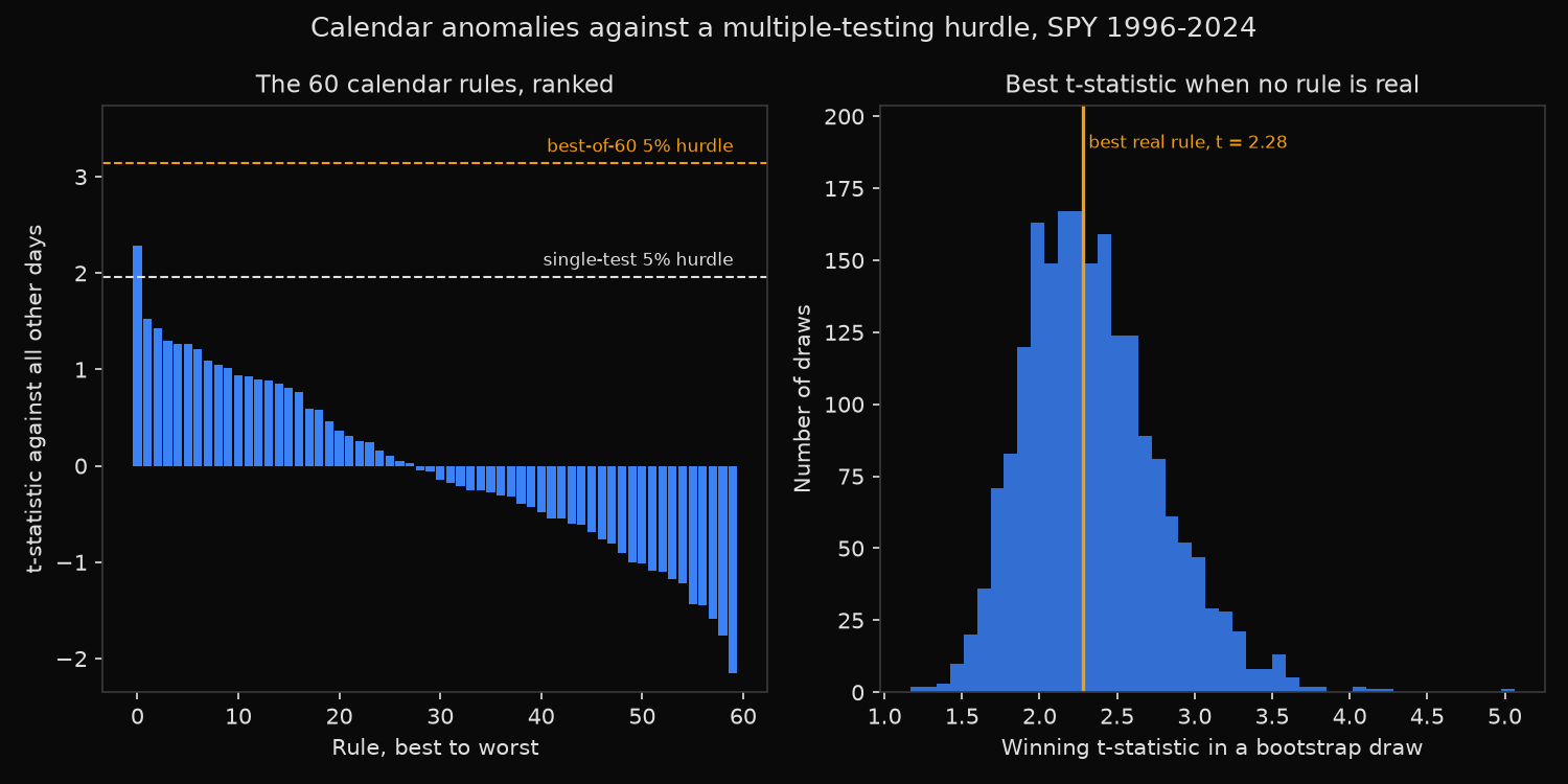
The SPY winner looks publishable: April Thursdays returned 0.252% per day across 124 days, the t-statistic is 2.28, and the single-test p-value of 0.0225 clears the conventional 5% screen. Measured against the search that produced it, the same rule carries a p-value of 0.5105: more than half of the bootstrap searches found a better rule in data where no rule exists.

The hurdle explains why. Under the null, the best of 60 rules reaches t = 3.14 one time in twenty, against 1.96 for a rule fixed in advance. A Šidák correction for 60 independent tests puts the same one-sided threshold at 3.14, confirming the bootstrap is calibrated, not merely pessimistic.

The wider family agrees. SPY produced 2 rules with an absolute t above 1.96 where 3.0 are expected by chance, QQQ exactly 3, IWM 1. The QQQ winner tempts hardest at 0.517% per day with a single-test p-value of 0.0203, yet its adjusted p-value of 0.4840 lands beside the SPY figure, and IWM reached 0.9875.

The method is not simply incapable of finding anything. A planted 0.25% per day went missing, at an adjusted p-value of 0.5770, and the contaminated September Tuesday cell did not even win its own search. At 0.50% per day the procedure worked, promoting Sep-Tue to winner with a t-statistic of 3.42 and an adjusted p-value of 0.0180. Real effects are found; they have to be twice the size of the SPY winner.

So what?

Correct the hurdle for the number of rules tried, not the number reported. A t-statistic of 2.28 on one pre-specified rule is evidence; the same 2.28 as the survivor of a sixty-way search is beaten by half of all searches run on noise, and no narrative about April tax flows changes that. Anyone reviewing an outside backtest should ask how many variants were run before this one was shown; that count sets the threshold.

The power check carries the more useful number for research design. A month-by-weekday cell holds roughly four days a year, so 29 years of history leaves the smallest SPY cell at 88 observations, and a sample that size resolves only effects near half a percent per day once the search is priced in. An effect half that size stays invisible here. Finding one needs a rule specified before the data are touched, which restores the 1.96 hurdle, or far more observations behind each candidate.

Both corrections cost about fifteen lines of code, and running them before capital moves is cheaper than learning the same thing from a live track record.

Built with xfinlink — free financial data API for Python. pip install -U xfinlink