How Long Does a Volatility Spike Take to Fade? Half-Life Estimation in Python

September 7, 2026

What’s the question?

After a stock’s volatility jumps, how long does it take to settle back to normal? The answer sets the fair price of every option written on that stock and the moment a volatility-targeted book can safely re-lever.

The standard way to answer it is a first-order autoregression, or AR(1), fitted to log realised volatility. Realised volatility is the standard deviation of returns actually observed over a block of days, as distinct from the volatility implied by option prices. An AR(1) states that each period equals a long-run average plus a fraction φ of the previous period’s deviation from it, plus noise. The half-life follows directly: ln(0.5)/ln(φ) periods pass before half the deviation is gone.

One number, easy to quote, and it is what one-factor stochastic volatility models such as Heston assume. The assumption carries a requirement that is rarely checked. If volatility genuinely follows an AR(1), the half-life expressed in trading days cannot depend on whether volatility was measured in weekly, fortnightly or monthly blocks. Sample the same process at four frequencies and the four answers should agree.

The approach

1. Pull ten years of split-adjusted daily closes for the current S&P 500 roster plus SPY, 2 September 2016 to 4 September 2026, or 2,515 trading days. Names without continuous trading across the window drop from the sample, as do seven carrying a single-day move above +100% or below -50%, which marks a corporate action rather than a return. That leaves 381 stocks.
2. Compute annualised realised volatility over non-overlapping blocks of 5, 10, 21 and 42 trading days, then take logs.
3. At each block length, estimate φ by pooled least squares with one mean per name, and convert it into a half-life in trading days.
4. Separately, find every week in which a stock’s realised volatility fell in its own top 5%, then track the median path of volatility over the following 52 weeks. No model is imposed here.
5. Compare that path against the AR(1) forecast, and convert the gap into the share of a spike an option of a given maturity ought to price.

Step 4 exists to check step 3. A regression slope can be dragged downward by estimation noise in the volatility measure itself, since five squared daily returns are a noisy read on a week’s true variance. An event path carries no such bias, so agreement between the two is evidence and disagreement is a finding.

Code

import time
import numpy as np
import pandas as pd
import xfinlink as xfl
from concurrent.futures import ThreadPoolExecutor

xfl.set_api_key("YOUR_API_KEY")  # free at https://xfinlink.com/signup

names = [t for t in sorted(xfl.index("sp500")["ticker"].unique()) if "-" not in t] + ["SPY"]

def grab(t):
    for a in range(4):
        try:
            return xfl.prices(t, start="2016-09-01", end="2026-09-04", fields=["adj_close"])
        except Exception:
            time.sleep(2 * (a + 1))
    return pd.DataFrame()

with ThreadPoolExecutor(4) as ex:
    px = pd.concat([d for d in ex.map(grab, names) if len(d)], ignore_index=True)

P = (px[px["ticker"].isin(names)].drop_duplicates(["ticker", "date"])
       .pivot(index="date", columns="ticker", values="adj_close").sort_index())
R = P.reindex(P["SPY"].dropna().index).pct_change().iloc[1:]
R = R.loc[:, R.notna().all()]
R = R.drop(columns=R.columns[((R > 1.0) | (R < -0.5)).any()])  # corporate-action artefacts
S = R.drop(columns="SPY")

def rvol(X, h):                      # annualised realised vol, non-overlapping h-day blocks
    nb = len(X) // h
    return np.sqrt((252.0 / h) * (X.iloc[:nb * h] ** 2)
                   .groupby(np.repeat(np.arange(nb), h)).sum())

def pooled_phi(L):                   # AR(1) slope, one mean per name
    D = L - L.mean()
    x0, x1 = D.iloc[:-1].values.ravel(), D.iloc[1:].values.ravel()
    return float((x0 @ x1) / (x0 @ x0))

for h in [5, 10, 21, 42]:
    phi = pooled_phi(np.log(rvol(S, h)))
    print(h, round(phi, 4), round(h * np.log(0.5) / np.log(phi), 1))

LW, K = np.log(rvol(S, 5)), [0, 1, 2, 4, 8, 13, 26, 52]
phi_w, mu = pooled_phi(LW), LW.mean()
act = {k: [] for k in K}
mod = {k: [] for k in K}
for c in LW.columns:
    y = LW[c].values
    hit = np.where(y >= np.quantile(y, 0.95))[0]
    for t in hit[hit + 52 < len(y)]:
        for k in K:
            act[k].append(np.exp(y[t + k] - mu[c]))
            mod[k].append(np.exp(phi_w ** k * (y[t] - mu[c])))

for k in K:
    print(k, round(float(np.median(act[k])), 2), round(float(np.median(mod[k])), 2))

s0 = np.log(np.median(act[0]))
frac = [np.log(np.median(act[k])) / s0 for k in K]
for N in [1, 4, 13, 26, 52]:
    ks = np.arange(1, N + 1)
    print(N, round(float(np.interp(ks, K, frac).mean()), 3),
          round(float(np.mean(phi_w ** ks)), 3))

Full script with formatting and visualisation: volatility-shock-half-life-python.py

Output

Sample: 381 S&P 500 stocks plus SPY, 2515 trading days, 2016-09-02 to 2026-09-04

AR(1) HALF-LIFE OF LOG REALISED VOLATILITY, BY SAMPLING HORIZON
  block  obs/name  phi (stocks)   half-life  phi (SPY)   half-life
    5d       503        0.3563      3.4d     0.5939      6.7d
   10d       251        0.4207      8.0d     0.6272     14.9d
   21d       119        0.4287     17.2d     0.6182     30.3d
   42d        59        0.4245     34.0d     0.4795     39.6d

DECAY AFTER A TOP-5% VOLATILITY WEEK (8768 stock-weeks)
weeks after    actual     AR(1)  spike left   ex-market
          0     3.13x     3.13x      100.0%       2.94x
          1     1.67x     1.50x       44.7%       1.28x
          2     1.50x     1.16x       35.8%       1.19x
          4     1.39x     1.02x       29.1%       1.15x
          8     1.28x     1.00x       21.3%       1.13x
         13     1.24x     1.00x       18.5%       1.18x
         26     1.17x     1.00x       14.0%       1.11x
         52     1.02x     1.00x        1.8%       1.03x
Excluding the 5% of weeks when SPY itself spiked: 5049 stock-weeks.

SHARE OF A SPIKE AN OPTION OF N WEEKS SHOULD PRICE
 maturity   actual   vol x    AR(1)   vol x
       1w    0.447   1.36x    0.356   1.28x
       4w    0.355   1.28x    0.136   1.10x
      13w    0.260   1.20x    0.043   1.03x
      26w    0.210   1.16x    0.021   1.01x
      52w    0.144   1.10x    0.011   1.01x

What this tells us

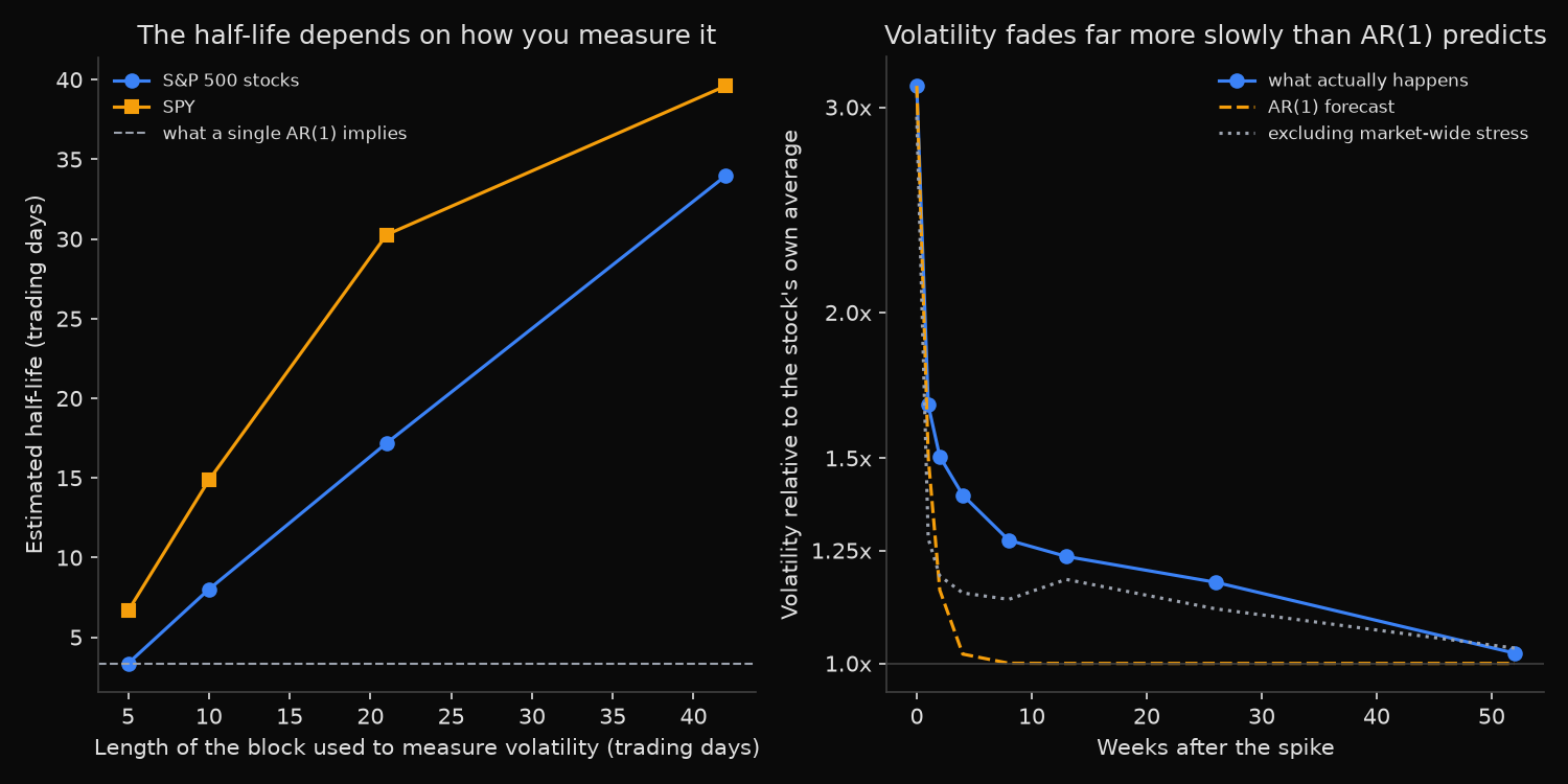
The half-life is not one number. Weekly blocks give 3.4 trading days, fortnightly blocks 8.0, monthly blocks 17.2, two-month blocks 34.0. Each estimate lands between 0.67 and 0.82 times the block that produced it, so the answer tracks the measurement window. A process that truly followed an AR(1) would return the same figure four times.

The event study shows what the regression misses. A week in the top 5% of a stock’s own volatility distribution runs at 3.13 times that stock’s average level, and a week later the median has dropped to 1.67 times, a fast collapse the AR(1) tracks passably at 1.50. Then the two separate. The AR(1) is back at its average by week four, while the observed median is still 1.39 there, 1.24 at week thirteen and 1.17 at week twenty-six; 14.0% of the spike survives half a year in log terms.

A steep initial fall followed by a long, flat tail is the signature of long memory: volatility has no single time scale, so fitting one scale forces a compromise, and the sampling window decides which compromise gets estimated.

Market-wide crises do not explain it. Dropping every week in which SPY’s own volatility sat in its top 5% leaves 5,049 idiosyncratic spikes, which rebound faster at first, 1.28 times after one week against 1.67, yet still sit 11% to 18% above average from week four through week twenty-six, where the AR(1) says zero.

SPY is the more persistent of the two at every block length, 6.7 days against 3.4 weekly and 30.3 against 17.2 monthly, because diversification cancels the company-specific shocks that decay fastest.

So what?

The cost of the wrong model sits in the last table. Take a stock whose volatility has just doubled. A one-factor model calibrated on weekly data says a three-month option should price 4.3% of that shock, raising fair volatility by 3%; the path volatility actually follows says 26.0%, raising it by 20%. At one year the comparison is 1.1% against 14.4%. A term structure quoted off a single mean-reversion speed sells long-dated volatility too cheaply in the weeks after a spike.

So calibrate the decay at the horizon being traded rather than borrowing an estimate from a different sampling frequency, and prefer a specification carrying several decay speeds, such as a HAR model that blends daily, weekly and monthly volatility. Volatility-target rules that assume a return to normal within a month re-lever early: a quarter after a spike the typical stock still runs about 24% hot.

The test is cheap. Fit the same AR(1) at four block lengths and check whether the half-lives agree; if they do not, the model has been rejected before a price is quoted.

Built with xfinlink — free financial data API for Python. pip install -U xfinlink