Do High-Accrual Companies Underperform? Accruals Screening in Python

August 28, 2026

What’s the question?

Accruals are the part of reported profit that did not arrive as cash. A company records revenue when it is earned rather than when the customer pays, and it records expenses when they are incurred rather than when the bill is settled. Net income and operating cash flow therefore diverge, and the size of that gap is the accrual component of earnings.

Richard Sloan showed in 1996 that the gap predicted stock returns. Companies whose profits leaned heavily on accruals went on to deliver lower returns than companies whose profits arrived as cash. The explanation offered was that investors treat both kinds of profit as equally durable, when accruals in fact reverse more often: a receivable that never converts, an inventory build that has to be written down, a deferred cost that eventually lands on the income statement.

Thirty years have passed, and the result is now taught in most quantitative finance courses. Anomalies published in academic journals tend to weaken once enough capital trades against them. The question here is narrow. Does an accruals sort still separate future winners from future losers among large US companies?

The approach

The accruals ratio used here is net income minus operating cash flow, divided by average total assets, where average total assets is the mean of the current and prior fiscal year values. Scaling by assets makes the measure comparable across companies of very different sizes.

1. Rebuild the S&P 500 roster as it stood at each year end from 2014 to 2024, so the sample holds the companies that were in the index at the time rather than the ones that survived to today.
2. Compute the accruals ratio for every company-year in that universe.
3. Form portfolios four months after each fiscal year closes, by which point the annual report has been filed and the inputs are public.
4. Measure the equal-weighted return over the following twelve months.
5. Sort each formation year into quintiles by accruals and compare the forward returns.

Winsorising at the 1st and 99th percentiles within each formation year stops a small number of extreme observations, mostly bankruptcy emergences and large asset writedowns, from dominating the averages. The final sample holds 4,751 company-years across 645 companies, formed between 2015 and 2024.

Code

import xfinlink as xfl
import pandas as pd

xfl.set_api_key("YOUR_API_KEY")  # free at https://xfinlink.com/signup

rosters = {y: set(xfl.index("sp500", as_of=f"{y}-12-31")["entity_id"])
           for y in range(2014, 2025)}
universe = sorted(set().union(*rosters.values()))

fund = xfl.fundamentals(entity_id=universe, start="2012-01-01", end="2026-08-01",
                        period_type="annual", max_rows=60000,
                        fields=["net_income", "operating_cash_flow", "total_assets"])
fund["period_end"] = pd.to_datetime(fund["period_end"])
fund = fund.sort_values(["entity_id", "period_end"])

fund["assets_lag"] = fund.groupby("entity_id")["total_assets"].shift(1)
fund["avg_assets"] = (fund["total_assets"] + fund["assets_lag"]) / 2
fund["accruals"] = (fund["net_income"] - fund["operating_cash_flow"]) / fund["avg_assets"]

# portfolios form four months after the fiscal year closes, by which point
# the annual report is public
fund["formation"] = fund["period_end"] + pd.DateOffset(months=4)
fund["form_year"] = fund["formation"].dt.year

# fwd12 is the twelve-month return from each formation date, compounded from
# daily returns pulled with xfl.prices(entity_id=universe, ...)
fund["fwd12"] = forward_returns(fund["entity_id"], fund["formation"])

fund["accruals_w"] = fund.groupby("form_year")["accruals"].transform(
    lambda s: s.clip(*s.quantile([0.01, 0.99])))
fund["quintile"] = fund.groupby("form_year")["accruals_w"].transform(
    lambda s: pd.qcut(s, 5, labels=[1, 2, 3, 4, 5]))

print(fund.groupby("quintile")["fwd12"].mean())

Full script with formatting and visualisation: do-high-accrual-companies-underperform-python.py

Output

firm-years 4,751  entities 645  2015-2024

forward 12-month return by accruals quintile (1 = lowest accruals)
          firm_years  mean_accruals  mean_fwd12  median_fwd12
quintile
1                956         -11.04       12.84          9.16
2                948          -5.59        9.80          7.96
3                948          -3.61        9.74          6.63
4                948          -1.88       10.96          9.20
5                951           1.80       10.93          8.56

Q1 minus Q5, averaged over formation years: 1.87pp
t-statistic 0.80   p-value 0.447   positive in 5 of 10 years

What this tells us

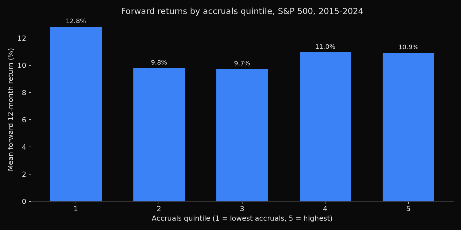
The sort produces the right sign and an unconvincing magnitude. Lowest-accrual companies returned 12.84% over the following year against 10.93% for the highest-accrual group, a gap of 1.91 percentage points in the pooled means and 1.87 points when each formation year is weighted equally. The t-statistic of 0.80 and p-value of 0.447 place that difference comfortably inside what random variation produces. The spread favoured low accruals in 5 of 10 formation years, which is a coin toss.

The shape of the sort is more damaging to the strategy than the significance test. A signal that works should grade: each quintile should sit between its neighbours. This one does not. Quintiles 2 and 3 returned 9.80% and 9.74%, below quintiles 4 and 5 at 10.96% and 10.93%. Only the extreme low-accrual quintile stands apart from the rest, and a single bucket separating itself while the ordering collapses in the middle is the signature of noise rather than a monotonic relationship.

Median returns tell the same story. The medians run 9.16%, 7.96%, 6.63%, 9.20% and 8.56%, with no ordering at all.

The accruals ratio itself behaves exactly as accounting theory predicts. It runs from an average of −11.04% of assets in the lowest quintile to +1.80% in the highest, and the negative average across most of the sample reflects depreciation, which pushes reported profit below operating cash flow for the majority of established companies. The measure is sound. What has gone is its ability to rank future returns in this universe.

Sloan’s original tests ran on the full cross-section of US listed companies, where the effect concentrated in small, thinly traded names that were expensive to arbitrage. The S&P 500 is the opposite environment: the most heavily analysed segment of the market, where any published, easily computed signal is priced quickly.

So what?

An accruals screen should not carry weight as a standalone return signal in large-cap equities. Ranking the S&P 500 on this ratio and buying the cheapest decile is a strategy with no statistical support over the past decade, and the flat middle of the sort means that even the direction is unreliable for most of the universe.

The ratio keeps its diagnostic value, which is a different job. A company reporting rising profits while operating cash flow stalls is worth reading more closely, because the divergence has to resolve one way or the other. Used that way, accruals belong in a quality composite alongside measures such as debt levels and margin stability, or as a filter that flags names for further work, rather than as the ranking that decides allocation.

Two conditions would change the conclusion. Extending the universe below large caps reintroduces the illiquid names where the effect was originally strongest, and separating accruals into working-capital and non-current components sometimes restores predictive power that the combined measure loses. Both are testable on the same panel, and both should be tested before any capital follows an accruals sort.

Built with xfinlink — free financial data API for Python. pip install -U xfinlink