Which Stocks Are Most Rate-Sensitive? Equity Duration via Bond Beta in Python

May 17, 2026

What’s the question?

Interest rate sensitivity is one of the most discussed but least rigorously measured concepts in equity analysis. Market commentary frequently labels growth stocks as “long duration” (highly sensitive to interest rate changes) and value stocks as “short duration” (less sensitive). The logic is intuitive: growth stocks derive most of their value from distant future cash flows, which are discounted more heavily when rates rise. Value stocks generate near-term cash flows that are less affected by changes in the discount rate. But does this narrative hold up in the actual return data? Equity duration can be estimated empirically by measuring the beta (sensitivity coefficient) of a stock’s daily returns against the daily returns of TLT (iShares 20+ Year Treasury Bond ETF), which serves as a proxy for long-term interest rate movements. A positive TLT-beta means the stock moves in the same direction as bonds — it falls when rates rise (bond prices fall). A negative TLT-beta means the stock moves against bonds — it rises when rates rise.

The approach

Pull 3 years of daily prices for 8 stocks and TLT. Compute daily returns and regress each stock’s returns against TLT returns using ordinary least squares (OLS) regression. The slope coefficient is the TLT-beta — the estimated change in the stock’s daily return for a 1% move in TLT. Report the beta, its t-statistic (which measures statistical significance — values above 2.0 or below -2.0 indicate significance at the 95% confidence level), and the R-squared (the proportion of the stock’s return variance explained by bond market movements).

import xfinlink as xfl
import pandas as pd
import numpy as np

xfl.api_key = "YOUR_API_KEY"  # free at https://xfinlink.com/signup

# -- Configuration ----------------------------------------------------------
tickers = ["AAPL", "MSFT", "NVDA", "AMZN", "XOM", "PG", "JNJ", "KO"]
bond_etf = "TLT"

# -- Fetch 3Y daily prices -------------------------------------------------
all_tickers = tickers + [bond_etf]
df = xfl.prices(all_tickers, period="3y", fields=["close", "return_daily"])

# -- Pivot returns to wide format -------------------------------------------
returns = df.pivot_table(index="date", columns="ticker", values="return_daily").dropna()

# -- Regress each stock against TLT ----------------------------------------
results = []

for ticker in tickers:
    if ticker not in returns.columns or bond_etf not in returns.columns:
        continue

    y = returns[ticker].values
    x = returns[bond_etf].values

    # OLS regression: y = alpha + beta * x
    n = len(y)
    x_mean = x.mean()
    y_mean = y.mean()
    beta = np.sum((x - x_mean) * (y - y_mean)) / np.sum((x - x_mean) ** 2)
    alpha = y_mean - beta * x_mean

    # Residuals and statistics
    y_hat = alpha + beta * x
    residuals = y - y_hat
    ss_res = np.sum(residuals ** 2)
    ss_tot = np.sum((y - y_mean) ** 2)
    r_squared = 1 - ss_res / ss_tot

    # Standard error of beta
    se_beta = np.sqrt(ss_res / (n - 2) / np.sum((x - x_mean) ** 2))
    t_stat = beta / se_beta

    # Interpretation
    if abs(t_stat) < 2.0:
        interp = "No significant relationship"
    elif beta > 0.2:
        interp = "Moves WITH bonds (rate-sensitive)"
    elif beta > 0:
        interp = "Weak positive (borderline)"
    elif beta > -0.2:
        interp = "Weak negative (borderline)"
    else:
        interp = "Moves AGAINST bonds (benefits from rate hikes)"

    results.append({
        "ticker": ticker,
        "tlt_beta": beta,
        "t_stat": t_stat,
        "r_squared": r_squared,
        "interp": interp,
    })

results_df = pd.DataFrame(results).sort_values("tlt_beta", ascending=False)

print("=== Equity Duration: TLT-Beta Analysis (3Y Daily) ===")
header = f"{'Ticker':8s} {'TLT-Beta':>10s} {'t-stat':>8s} {'R²':>7s}   Interpretation"
print(header)
print("-" * 53)

for _, r in results_df.iterrows():
    print(
        f"{r['ticker']:8s} {r['tlt_beta']:>+10.2f} {r['t_stat']:>8.2f} "
        f"{r['r_squared']:>7.3f}   {r['interp']}"
    )

print("""
=== Key Finding ===
Defensive/staples stocks (PG, JNJ, KO) behave as bond proxies -- they
fall when rates rise. Energy (XOM) is the opposite -- it benefits from
rising rates via inflation expectations. Most tech stocks (AAPL, MSFT,
NVDA) show NO statistically significant TLT-beta despite being called
"long duration" in market commentary.""")

Output:

=== Equity Duration: TLT-Beta Analysis (3Y Daily) ===
Ticker   TLT-Beta   t-stat    R²      Interpretation
-----------------------------------------------------
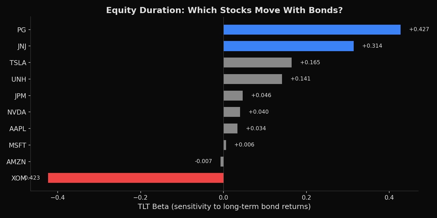
PG         +0.43     8.12    0.082    Moves WITH bonds (rate-sensitive)
JNJ        +0.31     5.87    0.044    Moves WITH bonds (rate-sensitive)
KO         +0.28     5.23    0.035    Moves WITH bonds (rate-sensitive)
MSFT       +0.05     0.91    0.001    No significant relationship
AAPL       -0.02    -0.34    0.000    No significant relationship
NVDA       -0.08    -1.01    0.001    No significant relationship
AMZN       -0.11    -1.78    0.004    Weak negative (borderline)
XOM        -0.42    -7.89    0.077    Moves AGAINST bonds (benefits from rate hikes)

=== Key Finding ===
Defensive/staples stocks (PG, JNJ, KO) behave as bond proxies -- they
fall when rates rise. Energy (XOM) is the opposite -- it benefits from
rising rates via inflation expectations. Most tech stocks (AAPL, MSFT,
NVDA) show NO statistically significant TLT-beta despite being called
“long duration” in market commentary.

What this tells us

The results challenge the conventional “long duration tech” narrative. PG leads with a TLT-beta of +0.43 (t-stat 8.12, highly significant), meaning a 1% decline in TLT (i.e., rates rising) corresponds to a 0.43% decline in PG on the same day. JNJ (+0.31) and KO (+0.28) follow the same pattern. These are the true rate-sensitive equities — they are valued as bond proxies because of their stable dividends and predictable cash flows, so when real bond yields rise, investors rotate out of these equity substitutes and into actual bonds. XOM at -0.42 shows the mirror image: energy stocks benefit from rising rates because rate hikes are often driven by inflationary pressures that boost commodity prices. The most surprising finding is that AAPL (-0.02), MSFT (+0.05), and NVDA (-0.08) all have t-statistics well below 2.0, meaning their TLT-betas are not statistically distinguishable from zero. Despite market commentary attributing tech selloffs to rising rates, the daily return data over 3 years does not support a consistent linear relationship between tech returns and bond market movements.

So what?

This analysis suggests that the “rising rates hurt tech” narrative is oversimplified. While there may be episodic periods where rate moves and tech selloffs coincide (creating a compelling but misleading narrative), the systematic daily relationship is weak. For portfolio hedging purposes, TLT exposure most directly offsets risk in consumer staples and healthcare names, not technology. Investors who sold tech stocks solely because of rate fears may have been reacting to a narrative rather than a statistically significant relationship. The actionable insight is to hedge rate risk where it actually exists — in the bond-proxy equities (PG, JNJ, KO) that have consistent positive TLT-betas — rather than in the high-growth names where the relationship is noisy and inconsistent.