Does R&D Spending Predict Revenue Growth? Cross-Sectional Test in Python

August 17, 2026

What’s the question?

Research and development is the one large expense a company chooses to incur entirely for the future. Wages, rent and raw materials keep the current business running. R&D buys products that do not exist yet, and it depresses reported earnings today in exchange for revenue that may or may not arrive.

Investors treat that trade as an article of faith. A company spending a fifth of its revenue on engineering is described as investing in growth, and the market usually prices it accordingly. The claim is rarely tested on the numbers, which leaves an obvious question: among large US companies, does the amount spent on research actually forecast how fast revenue grows afterwards?

R&D intensity is the standard way to measure the commitment: research and development expense divided by revenue in the same year. It scales the spend so a $2 billion research budget at a $10 billion company counts as heavier than the same budget at a $100 billion one. The test below asks whether that ratio, known today, says anything about the three years that follow.

The approach

The sample covers current S&P 500 members that report a research and development line in their annual accounts, which is 249 companies. Members are identified by permanent entity id rather than ticker symbol, so a company that changed symbol during the period stays matched to its own history.

1. Pull annual revenue and R&D expense from 2016 through the most recent filings.
2. Map each fiscal year onto the calendar year it mostly covers, so a January year-end and a December year-end are compared on the same footing.
3. For every starting year from 2017 to 2022, compute R&D intensity in that year and the compound annual revenue growth over the following three years.
4. Sort companies into quintiles by intensity inside each starting year. Forming the groups within the year removes the effect of a strong or weak macroeconomic period, so quintile 5 is never simply the year when everything grew.
5. Pool the six starting years into 1,417 company-year observations and compare growth across quintiles.

The ordering is what makes the result interpretable. R&D intensity is measured in year t and growth from year t to year t+3, so the predictor is fixed before any of the outcome happens. A mechanical link running backwards, in which fast growth inflates the research budget, cannot produce the pattern.

Code

import numpy as np
import pandas as pd
from scipy import stats
import xfinlink as xfl

xfl.set_api_key("YOUR_API_KEY")  # free at https://xfinlink.com/signup

HORIZON = 3
members = xfl.index("sp500")
ids = members["entity_id"].dropna().astype(int).tolist()
frames = []
for i in range(0, len(ids), 100):
    frames.append(xfl.fundamentals(
        entity_id=ids[i:i + 100], period_type="annual", start="2016-01-01", end="2026-06-30",
        fields=["revenue", "research_and_development", "gics_sector"]))
f = pd.concat(frames, ignore_index=True)
f["period_end"] = pd.to_datetime(f["period_end"])
f["cy"] = f["period_end"].dt.year - (f["period_end"].dt.month <= 6).astype(int)
f = f[f["revenue"] > 0].sort_values(["entity_id", "cy"]).drop_duplicates(["entity_id", "cy"], keep="last")

rev = f.pivot(index="cy", columns="entity_id", values="revenue")
rd = f.pivot(index="cy", columns="entity_id", values="research_and_development")

obs = []
for t in range(2017, 2026 - HORIZON):
    d = pd.DataFrame({
        "intensity": rd.loc[t] / rev.loc[t],
        "growth": (rev.loc[t + HORIZON] / rev.loc[t]) ** (1 / HORIZON) - 1,
    }).dropna()
    obs.append(d[(d["intensity"] > 0) & (d["intensity"] < 1)].assign(t=t))
o = pd.concat(obs)

o["q"] = o.groupby("t")["intensity"].transform(lambda s: pd.qcut(s, 5, labels=False) + 1)
print(o.groupby("q")["growth"].median() * 100)
print(stats.spearmanr(o["intensity"], o["growth"]))

Full script with formatting and visualisation: rd-intensity-forward-revenue-growth-python.py

Output

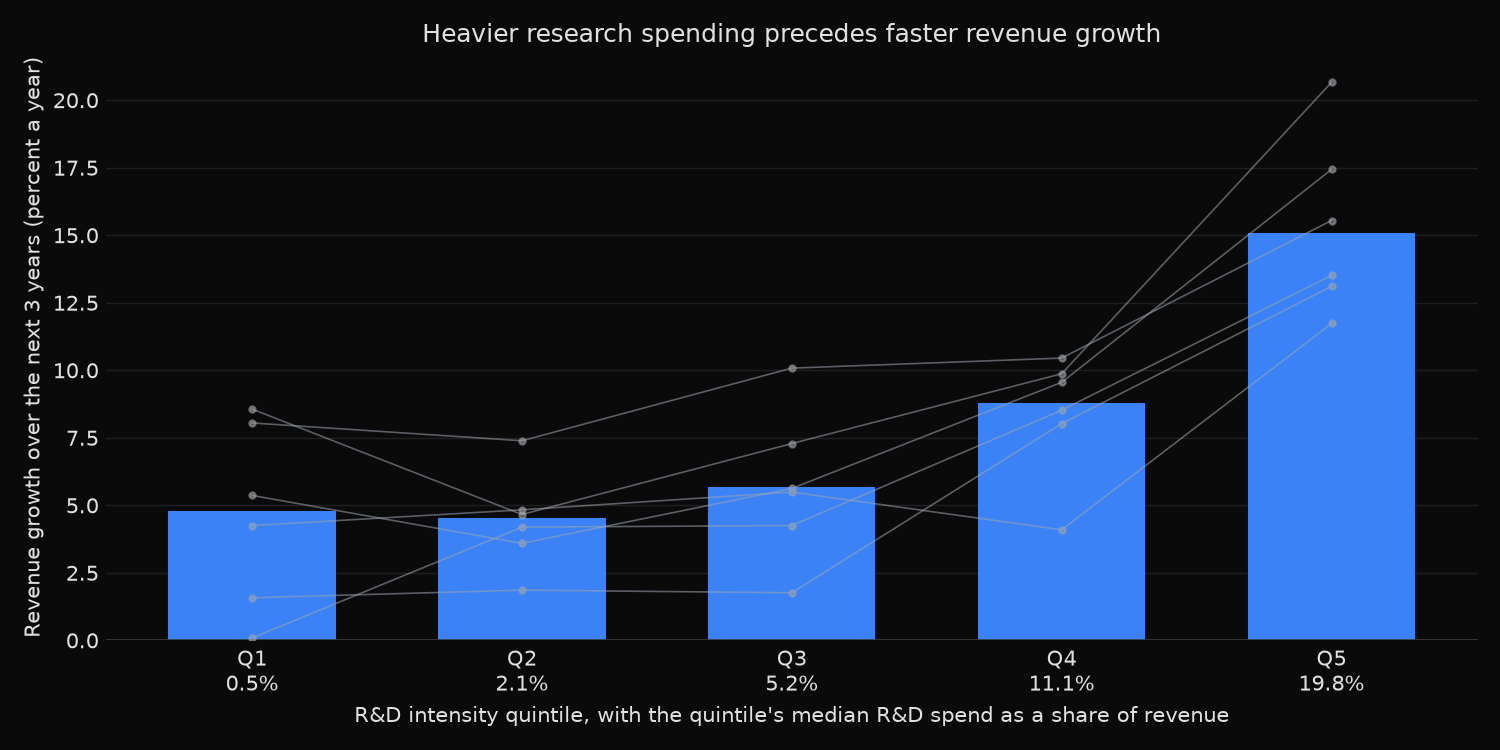
pooled observations: 1417, companies: 249

R&D intensity quintile -> revenue CAGR over the next 3 years (percent)
     n  rd_intensity  median_cagr  mean_cagr
q
1  286          0.51         4.79       5.74
2  282          2.14         4.54       8.08
3  281          5.16         5.67       6.68
4  282         11.07         8.79      10.22
5  286         19.79        15.09      18.71

pooled Spearman rho = 0.357 (p = 1.0e-43, n = 1417)

By starting year
  2017->2020  n=232  Q1  1.58%  Q5 13.11%  spread +11.53pp  rho +0.451
  2018->2021  n=239  Q1  5.37%  Q5 17.44%  spread +12.07pp  rho +0.423
  2019->2022  n=237  Q1  8.56%  Q5 20.66%  spread +12.10pp  rho +0.351
  2020->2023  n=240  Q1  8.05%  Q5 15.55%  spread +7.50pp  rho +0.230
  2021->2024  n=242  Q1  4.25%  Q5 11.73%  spread +7.48pp  rho +0.267
  2022->2025  n=227  Q1  0.09%  Q5 13.51%  spread +13.42pp  rho +0.452

Within sector (40 or more observations)
  Communication Services   n= 48  median intensity 13.11%  rho +0.268 (p=0.065)
  Consumer Discretionary   n= 77  median intensity  5.58%  rho +0.278 (p=0.014)
  Consumer Staples         n=130  median intensity  1.06%  rho -0.004 (p=0.961)
  Energy                   n= 81  median intensity  0.71%  rho +0.162 (p=0.149)
  Financials               n= 41  median intensity  6.93%  rho +0.100 (p=0.534)
  Health Care              n=243  median intensity  7.88%  rho +0.262 (p=0.000)
  Industrials              n=280  median intensity  2.57%  rho +0.100 (p=0.095)
  Information Technology   n=386  median intensity 13.36%  rho +0.460 (p=0.000)
  Materials                n=109  median intensity  1.37%  rho -0.058 (p=0.551)

What this tells us

The relationship is real and large. Companies in the heaviest-spending quintile, with a median research budget of 19.8 percent of revenue, went on to grow revenue at 15.1 percent a year over the following three years. The lightest spenders, at 0.5 percent of revenue, managed 4.8 percent. The gap of roughly ten percentage points a year compounds to a difference of about a third in cumulative revenue over three years.

The pattern is monotonic across the top three quintiles and flat across the bottom two. Moving from 0.5 percent of revenue to 2.1 percent changes nothing measurable, with median growth of 4.79 percent against 4.54 percent. Serious spending is where the separation happens: quintile 4 at 11.1 percent intensity reaches 8.8 percent growth, and quintile 5 doubles that again. A token research budget appears to buy nothing.

Consistency across starting years is what makes this more than a technology-boom artifact. All six cohorts show a positive spread, ranging from 7.5 to 13.4 percentage points, and the two widest gaps come from the 2017 and 2022 cohorts, whose outcome windows have almost nothing in common. The 2022 cohort is the strongest of all, with light spenders essentially flat at 0.09 percent a year while heavy spenders grew 13.5 percent.

The sector breakdown sharpens the claim considerably. Within Information Technology the rank correlation is 0.460, the highest anywhere, and within Health Care it is 0.262. Within Consumer Staples it is -0.004, which is nothing at all, and within Materials it is -0.058. Those two sectors spend around 1 percent of revenue on research. Where R&D is a genuine strategic lever, the amount spent separates the fast growers from the slow ones. Where research is a rounding error in the cost base, varying it changes nothing, and growth is decided by price, volume and distribution instead.

One caution belongs on the interpretation. The timing rules out reverse causation, but not selection: companies operating in expanding markets have both the opportunity and the cash to fund large research budgets, so part of the measured effect reflects which market a company happens to be in rather than what its spending achieved.

So what?

For screening, R&D intensity earns a place as a growth-forecasting variable in technology and healthcare, and deserves no weight at all in staples, materials or energy. Applying it uniformly across a whole index blends a strong signal with pure noise and dilutes both.

The threshold matters more than the ranking. Since the bottom two quintiles are indistinguishable, treating intensity as a continuous score wastes most of its information. A simple indicator for spending above roughly 10 percent of revenue captures nearly the whole effect, and it is more stable year to year than a percentile rank that shuffles companies around inside a flat region.

For valuation work, the number to carry forward is the ten-point growth gap. When a heavy spender trades at a premium multiple to a light spender in the same sector, that premium is not automatically excessive; the historical record says the faster revenue growth usually arrives. The question worth asking is whether the premium implies more growth than ten points a year, because that is roughly what the spending has bought.

Built with xfinlink — free financial data API for Python. pip install -U xfinlink