Is Residual Momentum Better Than Raw Momentum? Market-Adjusted Decile Sorts in Python

September 5, 2026

What’s the question?

Momentum ranks stocks on their own recent performance. The standard construction is 12-1: cumulative price return from twelve months ago to one month ago, skipping the last month because short-horizon reversal contaminates it. Buy the top decile, sell the bottom, hold a month, repeat.

A stock’s past return is not a clean measure of the stock. It contains whatever the market did over the same window, scaled by the stock’s beta, so a high-beta name in a rising market lands in the winner decile on the market’s strength rather than its own. Residual momentum removes that component before ranking: fit a market model to each stock, keep the residuals, and cumulate those. Does the resulting signal sort future returns better than the raw version, or was the market component carrying the signal all along?

The approach

The sample is the S&P 500 as it actually stood, from point-in-time rosters at 103 month ends between January 2018 and July 2026, covering 651 companies. Names are carried by entity id rather than ticker, so a recycled or changed symbol does not swap one company for another mid-test. Daily price returns start in June 2014, giving the market model history before the first sort.

1. At each month end, keep the names on that month’s roster with a complete daily series across the estimation window and the holding month. Both scores use the same names, so the comparison is like for like.
2. Raw score: cumulative log price return from 252 trading days before the sort date to 21 trading days before it.
3. Fit each name’s daily price returns on SPY daily price returns by ordinary least squares over the 756 trading days ending at the skip point.
4. Residual score: apply those coefficients over the 12-1 window and sum the residuals. The estimation window is three times the formation window, so those residuals do not sum to zero.
5. Sort into deciles on each score separately, hold equal-weighted for the next month, record top decile minus bottom decile.

Code

import numpy as np
import pandas as pd
import xfinlink as xfl

xfl.set_api_key("YOUR_API_KEY")  # free at https://xfinlink.com/signup

members = xfl.index("sp500", as_of="2024-12-31")["entity_id"].tolist()
px = xfl.prices(entity_id=members[:20], start="2019-01-01", end="2026-08-31",
                fields=["close", "return_daily"], max_rows=200000)
spy = xfl.prices("SPY", start="2019-01-01", end="2026-08-31", fields=["return_daily"])

R = px.pivot(index="date", columns="entity_id", values="return_daily").sort_index().dropna(axis=1)
mkt = spy.set_index("date")["return_daily"].reindex(R.index).values
logret = np.log1p(R.fillna(0.0)).cumsum().values

t = len(R) - 1                      # sort date
s, f, b = t - 21, t - 252, t - 777  # skip point, formation start, estimation start

X, mm = R.values[b + 1:s + 1], mkt[b + 1:s + 1]
md = mm - mm.mean()
beta = (X - X.mean(0)).T @ md / (md @ md)
alpha = X.mean(0) - beta * mm.mean()

raw = logret[s] - logret[f]                            # 12-1 cumulative price return
res = (R.values[f + 1:s + 1] - alpha - np.outer(mkt[f + 1:s + 1], beta)).sum(0)

decile = lambda x: np.argsort(np.argsort(x)) * 10 // len(x)
print(pd.DataFrame({"raw": decile(raw), "residual": decile(res)}, index=R.columns).head())

Full script with formatting and visualisation: residual-momentum-vs-raw-momentum-python.py

Output

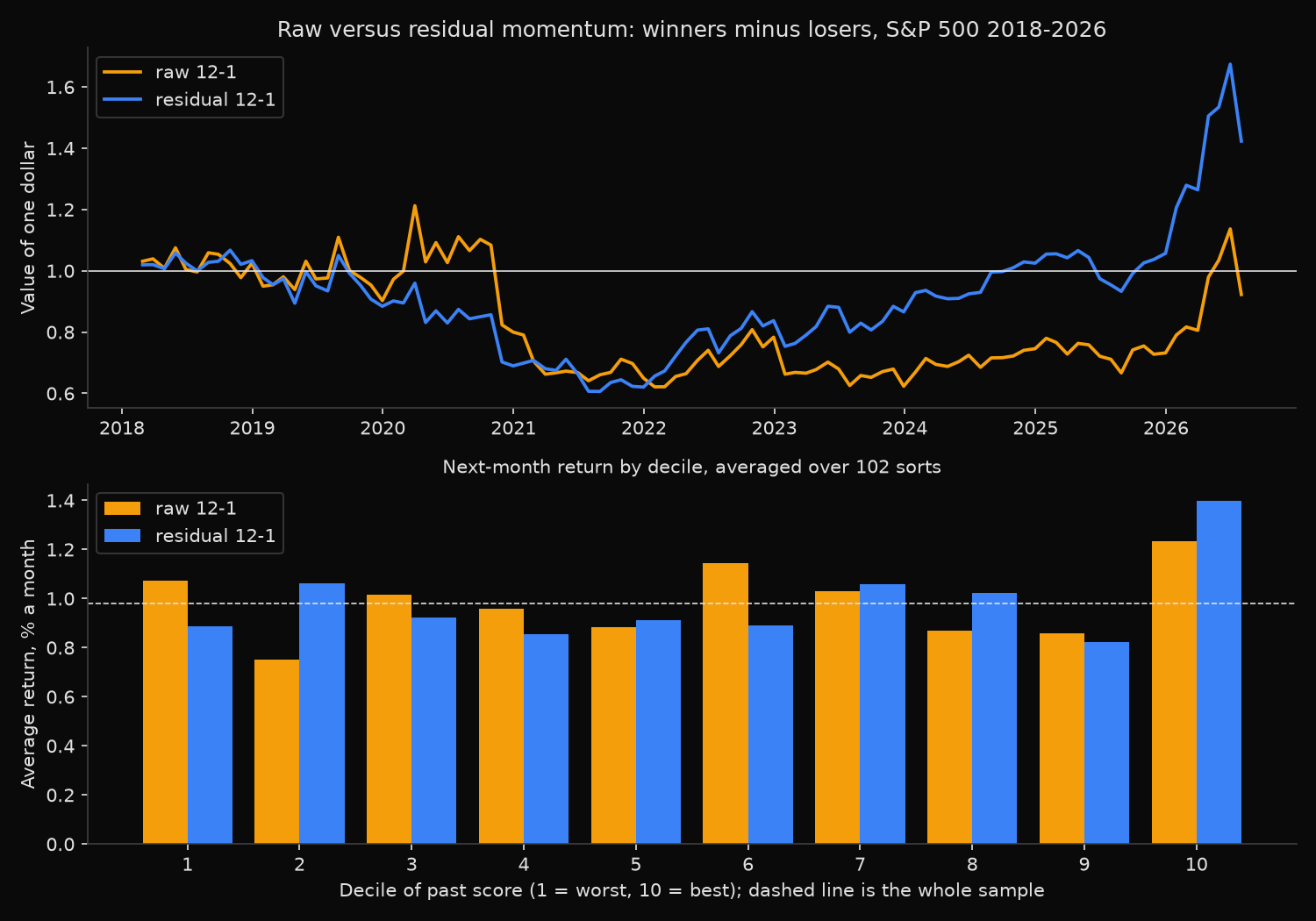
Raw versus residual 12-1 momentum, point-in-time S&P 500
Panel:    103 month-end rosters covering 651 companies; 649 carry a daily
          price series for the window and 631 remain after the return screen
Signals:  formation window 252 trading days ending 21 days before the sort date;
          market model fitted on the prior 756 trading days against SPY
Sorts:    102 monthly holding periods, 2018-02 to 2026-07, median 477 names ranked
          (range 442 to 482); equal-weighted top decile minus bottom decile

Signal          Monthly   A year      Vol   Sharpe       t   Hit rate   $1 becomes
Raw 12-1         0.158%   -0.94%   23.75%     0.08    0.23      53.9%         0.92
Residual 12-1    0.510%    4.24%   19.82%     0.31    0.90      57.8%         1.42

Legs of each spread, average monthly return
  Raw winners         1.232%   a year  13.58%   vol  20.21%   Sharpe  0.73
  Raw losers          1.074%   a year   8.79%   vol  29.73%   Sharpe  0.43
  Residual winners    1.397%   a year  15.85%   vol  19.91%   Sharpe  0.84
  Residual losers     0.887%   a year   7.44%   vol  26.48%   Sharpe  0.40
  Whole sample        0.982%   a year  10.66%   vol  17.91%   Sharpe  0.66

How far apart are the two rankings?
  Mean rank correlation of the two scores    0.816   (0.712 to 0.891)
  Top decile shared by both signals          61.7%   (36.2% to 81.8%)
  Correlation of the two monthly spreads     0.843
  Residual minus raw, mean monthly          0.352%   (t = 0.96)

Market exposure carried into the long-short book
  Rank correlation of score with beta       raw +0.020   residual -0.034
  Net beta of winners minus losers, mean    raw +0.059   residual -0.025
  Net beta, standard deviation across sorts raw  0.330   residual  0.245
  Net beta, range across sorts              raw -0.52 to +0.71   residual -0.49 to +0.57

Long-short return by calendar year
  Year      Raw   Residual
  2018    2.50%     3.30%
  2019  -11.93%   -14.41%
  2020  -11.39%   -21.99%
  2021  -18.79%   -10.03%
  2022   20.60%    34.93%
  2023  -20.44%     3.42%
  2024   19.65%    18.36%
  2025   -1.85%     3.13%
  2026   26.05%    34.64%
  Residual ahead in 6 of 9 calendar years

Average monthly return by decile (1 = worst past score, 10 = best)
  Decile            1      2      3      4      5      6      7      8      9     10
  Raw        1.07%  0.75%  1.02%  0.96%  0.88%  1.14%  1.03%  0.87%  0.86%  1.23%
  Residual   0.89%  1.06%  0.92%  0.85%  0.91%  0.89%  1.06%  1.02%  0.82%  1.40%

What this tells us

Residualising improved every summary statistic. The residual spread averaged 0.510% a month against 0.158% for the raw sort, at lower volatility (19.82% against 23.75%) and a higher hit rate (57.8% against 53.9%). Compounded over 102 months, one dollar in the raw spread ended at 0.92 against 1.42 for the residual spread. The 2018 and 2026 rows are part years.

Both legs improved, the short leg slightly more. The decile table shows how badly the raw short leg was placed: its bottom decile averaged 1.07% a month, more than seven of the nine deciles above it and more than the 0.982% sample average. The residual bottom decile came in at 0.89%, where a short leg belongs.

The beta rows explain the drop in volatility, and the explanation is not the obvious one. Across the 102 sorts the raw score is nearly uncorrelated with beta (rank correlation +0.020) and the raw book carries a mean net beta of +0.059, so raw momentum holds no persistent market tilt. It holds an unstable one: net beta swings from -0.52 to +0.71 across sorts, standard deviation 0.330, and residualising cuts that to 0.245 while leaving the average alone. The exposure wanders, flipping sign with whatever the market did over the past year, and that is what makes the raw spread the more volatile of the two.

Neither signal reaches statistical significance here: t-statistics of 0.23 on the raw spread, 0.90 on the residual spread, and 0.96 on the 0.352% monthly gap between them. The rankings agree on most names anyway, with a mean rank correlation of 0.816 and 61.7% of the top decile shared. Residual momentum is a tilt on raw momentum, not a different strategy, though where they diverge the gap is wide: in 2023 raw lost 20.44% and residual gained 3.42%.

So what?

The case for residualising rests on the exposure, not on the return gap. One regression per name per sort cut a quarter of the variability in the book’s market exposure, and that is a direct measurement rather than an inference drawn from noisy returns. The return advantage over these 102 months, 0.352% a month, is not statistically distinguishable from zero, so 4.24% a year against -0.94% is what this sample delivered, not what the adjustment can be expected to add.

Do not expect the adjustment to rescue a signal that is not working. Both spreads spent 2019 through 2021 underwater, and the residual version fell further in 2020 than the raw one did. Residualising narrows the volatility and shifts the average; it does not change the years when cross-sectional momentum stops paying.

Anyone hedging a raw momentum book to a fixed market exposure should check the net beta range first: a constant hedge assumes a constant exposure, and this one moved between -0.52 and +0.71. Residualising acts on the ranking instead of on the position after the fact.

Built with xfinlink — free financial data API for Python. pip install -U xfinlink