Do Companies Pay the Tax They Report? Cash vs Book Tax Rates in Python

September 4, 2026

What’s the question?

Every annual report carries two tax numbers. The income statement shows income tax expense, an accrual computed under accounting rules. The cash flow statement shows cash taxes paid, the money that actually left the company. Deferred tax accounting connects them, and the standard reading of that connection is timing: tax deferred in one year reverses in a later one, so the two converge over a long enough window.

That assumption does real work in valuation. A discounted cash flow model has to tax operating profit at some rate, and the rate most analysts reach for is the reported effective rate, which sits on the face of the income statement; cash taxes paid sits further back in the supplemental disclosures and rarely reaches a screen. Where a company reports 21% and pays 4% for ten consecutive years, every forecast year built on the reported rate understates free cash flow.

The book effective tax rate is income tax expense over pretax income, and the cash tax rate is cash taxes paid over the same pretax income. This tests whether they meet across a decade.

The approach

The test window is fiscal 2014 through fiscal 2023, long enough for ordinary timing differences to unwind.

1. Build the universe from the point-in-time S&P 500 roster at each year end from 2013 to 2023, then take the union. Membership is carried by entity id, so a company that changed ticker during the decade keeps one continuous series.
2. Drop financials and real estate, whose tax and balance sheet mechanics do not compare with operating companies.
3. Keep only companies reporting ten consecutive profitable fiscal years, since a tax rate computed on a loss is not interpretable.
4. Sum pretax income, income tax expense and cash taxes paid across the ten years for each company, then divide. Summing first, rather than averaging ten annual ratios, stops one small-denominator year from dominating.
5. Compare the two rates in aggregate, across the firm-level distribution, and by sector.

Code

import pandas as pd
import xfinlink as xfl

xfl.set_api_key("YOUR_API_KEY")  # free at https://xfinlink.com/signup

ids = set()
for year in range(2013, 2024):
    ids |= set(xfl.index("sp500", as_of=f"{year}-12-31")["entity_id"])
ids = sorted(ids)

fields = ["revenue", "pretax_income", "income_tax_expense",
          "cash_taxes_paid", "net_income", "gics_sector"]
frames = [
    xfl.fundamentals(entity_id=ids[i:i + 100], period_type="annual",
                     start="2014-01-01", end="2024-06-30", fields=fields)
    for i in range(0, len(ids), 100)
]
df = pd.concat([f for f in frames if not f.empty], ignore_index=True)
df["fy"] = df["period_end"].dt.year - (df["period_end"].dt.month <= 5).astype(int)

d = df[~df["gics_sector"].isin(["Financials", "Real Estate"])].copy()
d = d.dropna(subset=["revenue", "pretax_income", "income_tax_expense",
                     "cash_taxes_paid"])
d = d[(d["revenue"] > 0) & (d["pretax_income"] > 0) & d["fy"].isin(range(2014, 2024))]
d = d.drop_duplicates(["entity_id", "fy"], keep=False)

counts = d.groupby("entity_id")["fy"].nunique()
d = d[d["entity_id"].isin(counts[counts == 10].index)]

# Sum by entity, not by ticker: one company can file under two symbols.
d = d.sort_values(["entity_id", "fy"])
labels = d.groupby("entity_id")[["ticker", "entity_name", "gics_sector"]].last()
firm = (d.groupby("entity_id")
          [["pretax_income", "income_tax_expense", "cash_taxes_paid"]]
          .sum().join(labels).reset_index())
firm["book_etr"] = firm["income_tax_expense"] / firm["pretax_income"]
firm["cash_etr"] = firm["cash_taxes_paid"] / firm["pretax_income"]
firm["gap_pp"] = (firm["book_etr"] - firm["cash_etr"]) * 100

sector = (firm.groupby("gics_sector")
               .agg(n=("ticker", "size"), book=("book_etr", "median"),
                    cash=("cash_etr", "median"))
               .assign(gap_pp=lambda t: (t["book"] - t["cash"]) * 100)
               .sort_values("gap_pp", ascending=False))

print(sector.round(3))
print(firm.nlargest(10, "gap_pp")[["ticker", "book_etr", "cash_etr", "gap_pp"]])

Full script with formatting and visualisation: cash-vs-book-tax-rate-python.py

Output

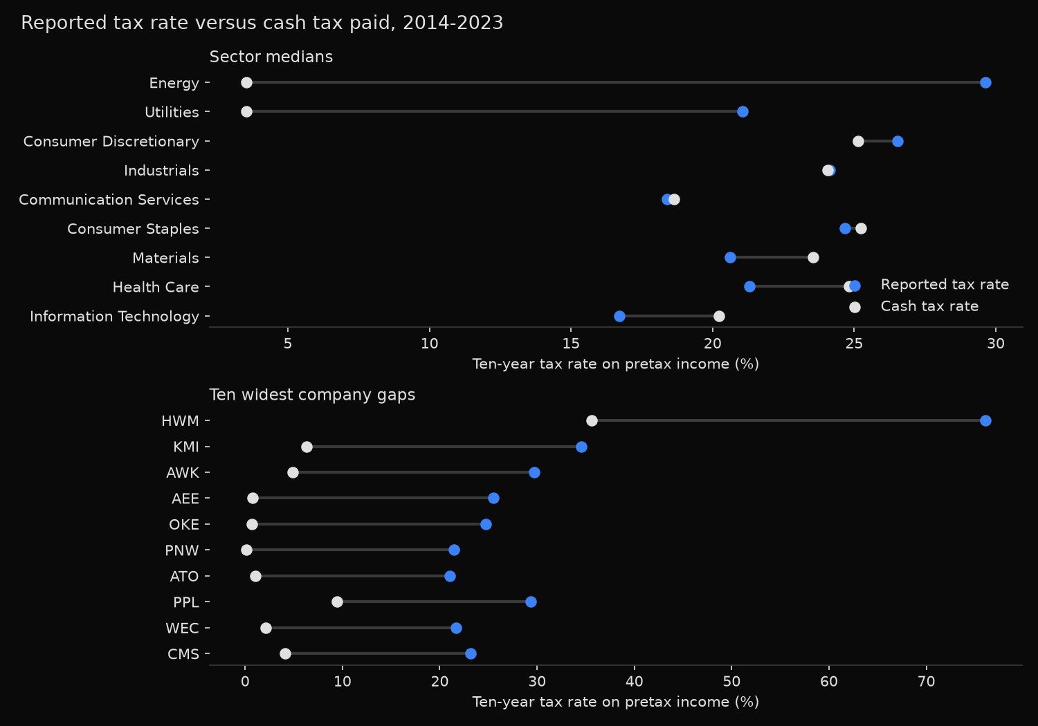
Companies with 10 straight profitable years (FY2014-FY2023): 248
Pretax income summed over the decade: $8.83tn
Aggregate book tax rate: 21.29%
Aggregate cash tax rate: 22.01%

Firm-level gap, book tax rate minus cash tax rate (percentage points)
  10th percentile:   -9.0
  25th percentile:   -3.6
  50th percentile:   -0.3
  75th percentile:   +2.1
  90th percentile:   +6.5
  Companies paying less than half their reported rate in cash: 21 of 248

Sector medians over the decade
Sector                     n    Book    Cash     Gap
Energy                     2   29.6%    3.5%   +26.1
Utilities                 19   21.1%    3.5%   +17.5
Consumer Discretionary    31   26.5%   25.1%    +1.4
Industrials               57   24.1%   24.1%    +0.1
Communication Services    10   18.4%   18.6%    -0.2
Consumer Staples          26   24.7%   25.2%    -0.6
Materials                 18   20.6%   23.5%    -2.9
Health Care               43   21.3%   24.8%    -3.5
Information Technology    42   16.7%   20.2%    -3.5

Ten widest decade gaps
Ticker  Sector                      Book    Cash     Gap
HWM     Industrials                76.1%   35.6%   +40.5
KMI     Energy                     34.5%    6.3%   +28.2
AWK     Utilities                  29.7%    4.9%   +24.8
AEE     Utilities                  25.5%    0.8%   +24.8
OKE     Energy                     24.7%    0.7%   +24.0
PNW     Utilities                  21.5%    0.1%   +21.3
ATO     Utilities                  21.1%    1.1%   +20.0
PPL     Utilities                  29.3%    9.4%   +19.9
WEC     Utilities                  21.7%    2.1%   +19.6
CMS     Utilities                  23.2%    4.1%   +19.0

What this tells us

At the level of the whole sample the textbook holds. Across 248 companies and $8.83tn of pretax income, the aggregate book rate of 21.29% and the aggregate cash rate of 22.01% differ by less than a point, because deferrals in one direction are cancelled by reversals elsewhere.

Individual companies are a different matter. The middle half of the distribution runs from 3.6 points of cash overpayment to 2.1 points of underpayment, the tenth percentile sits 9.0 points into overpayment and the ninetieth 6.5 points the other way, and 21 companies paid less than half their reported rate in cash across the full decade. That is too long a run to call timing.

Utilities carry the pattern: nineteen qualifying names show a median book rate of 21.1% against a median cash rate of 3.5%, and the two qualifying energy names sit in the same place. The mechanism is accelerated and bonus depreciation on capital spending, because a utility that keeps building rate base generates new tax depreciation faster than old deferrals reverse, so the deferred tax liability grows instead of unwinding. Pinnacle West booked 21.5% and paid 0.1% in cash; American Water Works reported 29.7% and paid 4.9%.

The gap runs the other way in Information Technology, which reports the lowest book rate of any sector at 16.7% and pays 20.2%. There the headline rate flatters the company, and a model taxing operating profit at the reported rate overstates free cash flow.

Howmet Aerospace tops the table for the opposite reason. Its 76.1% book rate comes from charges taken against thin pretax income during the Arconic separation years, including $1.48bn of tax expense on $414m of 2016 pretax income; the cash rate of 35.6% is the ordinary figure. Which side moved matters as much as the size of the gap.

So what?

Before setting the tax rate in a valuation model, compute the multi-year cash rate and compare it with the reported one; both numbers come from the same call. Where they agree, the reported rate is a fair proxy. Where they diverge by ten points or more, it is the wrong input: on $1bn of pretax income, a 17-point gap is $170m of cash a year.

That gap is not permanent by construction. It lasts only while the capital spending behind it lasts, so a forecast using the low cash rate has to carry the capital expenditure that earns it, and the terminal value has to converge back toward the statutory rate. Treating the low rate as free and permanent overvalues a utility as surely as ignoring it undervalues one.

For screening, the ratio of cumulative cash tax to cumulative book tax over ten years separates structural deferral from a single odd year. Below 0.5, look at the capital spending behind the deferred tax liability. Well above 1.0, look for the one-off charge that inflated the reported expense.

Built with xfinlink — free financial data API for Python. pip install -U xfinlink