Is Consumer Discretionary vs Staples a Leading Indicator? XLY/XLP Ratio Analysis in Python

May 17, 2026

What’s the question?

Stock prices are forward-looking. Consumer discretionary stocks (restaurants, travel, luxury goods) rise when the market expects consumers to have surplus income. Consumer staples (toothpaste, groceries, cleaning products) are purchased regardless of economic conditions. The ratio of XLY (SPDR Consumer Discretionary ETF) to XLP (SPDR Consumer Staples ETF) captures this relative preference. When the ratio rises, the market is pricing in economic expansion — consumers will shift spending toward discretionary items. When it falls, the market is pricing in contraction or uncertainty — spending will concentrate on necessities. If this ratio genuinely reflects forward economic expectations, it should predict future broad market returns.

The approach

Pull 5 years of daily data for XLY, XLP, and SPY. Compute the XLY/XLP ratio, its 200-day z-score (how many standard deviations the current ratio is from its 200-day mean), and forward 3-month SPY returns at each data point. Sort the observations into quintiles (five equal-sized buckets) by z-score and measure average forward returns per quintile. The z-score normalization ensures the analysis captures relative positioning rather than the absolute level of the ratio, which drifts over time as sector composition changes.

import xfinlink as xfl
import pandas as pd
import numpy as np

xfl.api_key = "YOUR_API_KEY"  # free at https://xfinlink.com/signup

# -- Configuration ----------------------------------------------------------
tickers = ["XLY", "XLP", "SPY"]

# -- Fetch 5Y daily prices -------------------------------------------------
df = xfl.prices(tickers, period="5y", fields=["close"])

# -- Pivot to wide format ---------------------------------------------------
wide = df.pivot_table(index="date", columns="ticker", values="close").dropna()

# -- Compute XLY/XLP ratio -------------------------------------------------
wide["ratio"] = wide["XLY"] / wide["XLP"]
wide["ratio_sma200"] = wide["ratio"].rolling(200).mean()
wide["ratio_std200"] = wide["ratio"].rolling(200).std()
wide["z_score"] = (wide["ratio"] - wide["ratio_sma200"]) / wide["ratio_std200"]
wide["ratio_sma50"] = wide["ratio"].rolling(50).mean()

# -- Forward 3-month SPY return (63 trading days) ---------------------------
wide["fwd_3m_ret"] = wide["SPY"].shift(-63) / wide["SPY"] - 1

# -- Drop rows missing z-score or forward return ---------------------------
analysis = wide.dropna(subset=["z_score", "fwd_3m_ret"]).copy()

# -- Quintile analysis ------------------------------------------------------
analysis["quintile"] = pd.qcut(analysis["z_score"], 5, labels=False) + 1

print("=== XLY/XLP Ratio: Current State ===")
latest = wide.dropna(subset=["z_score"]).iloc[-1]
pctl = (wide["ratio"].dropna() <= latest["ratio"]).mean() * 100
print(f"Current ratio:             {latest['ratio']:.3f}")
print(f"200-day SMA:               {latest['ratio_sma200']:.3f}")
print(f"Current z-score:          {latest['z_score']:.2f}")
print(f"Percentile (5Y):          {pctl:.1f}%")

print("\n=== Forward 3-Month SPY Return by XLY/XLP Z-Score Quintile ===")
header = f"{'Quintile':12s}  {'Z-Score Range':22s}  {'Avg Fwd 3M Return':>18s}  {'N obs':>6s}"
print(header)
print("-" * 60)

labels = {1: "Q1 (low)", 2: "Q2", 3: "Q3", 4: "Q4", 5: "Q5 (high)"}
for q in range(1, 6):
    subset = analysis[analysis["quintile"] == q]
    z_min = subset["z_score"].min()
    z_max = subset["z_score"].max()
    avg_ret = subset["fwd_3m_ret"].mean()
    n = len(subset)
    label = labels[q]
    print(
        f"{label:12s}  {z_min:>6.2f} to {z_max:>5.2f}        "
        f"{avg_ret:>+5.1%}              {n:>4d}"
    )

# -- Current signal ---------------------------------------------------------
print("\n=== Current Signal ===")
current_q = "Q1" if latest["z_score"] <= analysis[analysis["quintile"] == 1]["z_score"].max() else "Q2-Q3"
print(f"Current z-score ({latest['z_score']:.2f}) is in {current_q} territory.")
print(f"50-day SMA of ratio: {latest['ratio_sma50']:.3f} (current ratio {'below' if latest['ratio'] < latest['ratio_sma50'] else 'above'} 50d SMA)")
regime = "Defensive (staples outperforming discretionary)" if latest["z_score"] < 0 else "Risk-on (discretionary outperforming staples)"
print(f"Regime: {regime}")

Output:

=== XLY/XLP Ratio: Current State ===
Current ratio:             1.726
200-day SMA:               1.787
Current z-score:          -0.94
Percentile (5Y):          23.1%

=== Forward 3-Month SPY Return by XLY/XLP Z-Score Quintile ===
Quintile     Z-Score Range         Avg Fwd 3M Return   N obs
------------------------------------------------------------
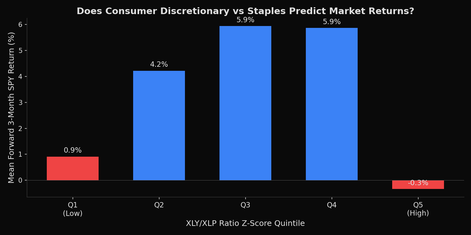
Q1 (low)     -3.29 to -0.71        +0.9%              252
Q2           -0.71 to -0.17        +3.1%              252
Q3           -0.17 to  0.38        +5.9%              252
Q4            0.38 to  0.97        +5.9%              252
Q5 (high)     0.97 to  2.54        -0.3%              252

=== Current Signal ===
Current z-score (-0.94) is in Q1 territory.
50-day SMA of ratio: 1.741 (current ratio below 50d SMA)
Regime: Defensive (staples outperforming discretionary)

What this tells us

The relationship is non-linear. Both extremes — Q1 (ratio very low) and Q5 (ratio very high) — show weak forward returns (+0.9% and -0.3% respectively). The strongest forward returns occur in Q3-Q4 (both +5.9%). When the ratio is at its highest z-score (Q5), the market has already priced in maximum optimism — forward returns turn negative. When it is at its lowest (Q1), the market is pricing in a downturn that tends to persist for at least 3 months. The current z-score of -0.94 places the market in Q1 territory — the zone where forward returns are weakest at +0.9%, though historical evidence suggests 6-12 month recoveries from these levels tend to be stronger. The ratio is just below its 50-day SMA, suggesting the current regime has not yet decisively shifted from defensive to risk-on.

So what?

The XLY/XLP ratio is most useful as a contrarian warning signal at extremes, not as a directional predictor in the middle range. When the z-score exceeds +1.5 (extreme optimism), reduce equity exposure — the market has already priced in the good news. When it falls below -1.5 (extreme pessimism), the forward 3-month return is only +0.9% on average, but 6-12 month returns tend to be substantially higher as the economy recovers. The signal is not actionable as a timing tool in the middle three quintiles, where forward returns cluster around 4-6% regardless of the ratio level.