Does Illiquidity Still Pay? Amihud Measure in the S&P 500 in Python

August 17, 2026

What’s the question?

An investor who buys a thinly traded stock accepts a cost that never appears on a statement: getting out again moves the price. Finance theory says that cost has to be compensated, otherwise nobody would hold the thin names. The illiquidity premium is the extra return expected for bearing it, and Amihud’s 2002 paper gave it a measure simple enough to compute from daily data.

The Amihud illiquidity ratio is the average of absolute daily return divided by daily dollar volume. It approximates price impact: how far the price moves per dollar traded. A stock whose price jumps 3 percent on $50 million of turnover is far less liquid than one that moves 0.5 percent on $800 million, and the ratio captures exactly that difference.

The premium is well documented across the whole US market, where the illiquid end contains genuine microcaps. Whether it survives inside the S&P 500 is a different question, and a more practical one for anyone running a large-cap mandate. Every member of that index is liquid in absolute terms. The least liquid member still turns over tens of millions of dollars a day. If the premium is a microcap phenomenon, it should vanish here.

The approach

The universe is the current S&P 500, addressed by permanent entity id so that a symbol change does not break the series. Daily closes, volumes and total returns run from June 2022 to December 2025.

1. Compute each stock’s daily illiquidity as the absolute daily return divided by that day’s dollar volume, then average within each month.
2. At the end of every month, rank stocks on the trailing twelve-month average of that measure and sort them into five equal groups.
3. Hold each group, equal weighted, for the following single month, then re-sort. This yields 30 monthly holding periods from July 2023 to December 2025.
4. Compare annualised return and annualised volatility across the groups, and test whether the return gap between the least and most liquid groups differs from zero.

Sorting monthly on a trailing average matters. Liquidity is not a fixed property of a company; it drifts with index membership, news and market conditions, so a signal fixed once at the start of the period would be measuring something stale by the end.

Code

import numpy as np
import pandas as pd
from scipy import stats
import xfinlink as xfl

xfl.set_api_key("YOUR_API_KEY")  # free at https://xfinlink.com/signup

members = xfl.index("sp500")
ids = members["entity_id"].dropna().astype(int).tolist()
parts = []
for i in range(0, len(ids), 50):
    parts.append(xfl.prices(entity_id=ids[i:i + 50], start="2022-06-01", end="2025-12-31",
                            fields=["close", "volume", "return_daily"], max_rows=400000))
px = pd.concat(parts, ignore_index=True)
px["date"] = pd.to_datetime(px["date"])

d = px.dropna(subset=["close", "volume", "return_daily"])
d = d[(d["volume"] > 0) & (d["close"] > 0)].copy()
d["illiq"] = d["return_daily"].abs() / (d["close"] * d["volume"])
d["month"] = d["date"].dt.to_period("M")

monthly = d.groupby(["entity_id", "month"]).agg(
    illiq=("illiq", "mean"),
    ret=("return_daily", lambda r: (1 + r).prod() - 1),
    n=("return_daily", "size")).reset_index()
monthly = monthly[monthly["n"] >= 15]

ill = monthly.pivot(index="month", columns="entity_id", values="illiq")
ret = monthly.pivot(index="month", columns="entity_id", values="ret")

months, rows = list(ill.index), []
for k in range(12, len(months) - 1):
    frame = pd.DataFrame({"signal": ill.loc[months[k - 11]:months[k]].mean(),
                          "fwd": ret.loc[months[k + 1]]}).dropna()
    frame["q"] = pd.qcut(frame["signal"], 5, labels=False) + 1
    g = frame.groupby("q")["fwd"].mean()
    rows.append(pd.DataFrame({"month": months[k + 1], "q": g.index, "fwd": g.values}))

piv = pd.concat(rows, ignore_index=True).pivot(index="month", columns="q", values="fwd")
print((1 + piv.mean()) ** 12 - 1)          # annualised return by quintile
print(piv.std(ddof=1) * np.sqrt(12))       # annualised volatility by quintile
print(stats.ttest_1samp(piv[5] - piv[1], 0))

Full script with formatting and visualisation: amihud-illiquidity-sp500-python.py

Output

holding months: 30  (2023-07 to 2025-12)

Quintile  median daily $ volume  annualised return  annualised volatility
   Q1         $   793.1m             18.05%              11.62%
   Q2         $   312.8m             14.19%              12.41%
   Q3         $   216.7m             15.02%              14.13%
   Q4         $   141.1m             16.53%              15.32%
   Q5         $    88.4m             28.67%              16.32%

Q5 minus Q1: 0.731% a month, 9.13% annualised
  t = 1.52, p = 0.141, 30 months, 18 of 30 positive
  95% confidence interval, monthly: -0.21% to +1.68%
  months needed for t=2 at this effect size and volatility: 52 (4.4 years)

volatility rises at 4 of 4 steps from Q1 to Q5  (rank correlation with quintile = 1.00)

What this tells us

Two results sit in that output, and they behave very differently.

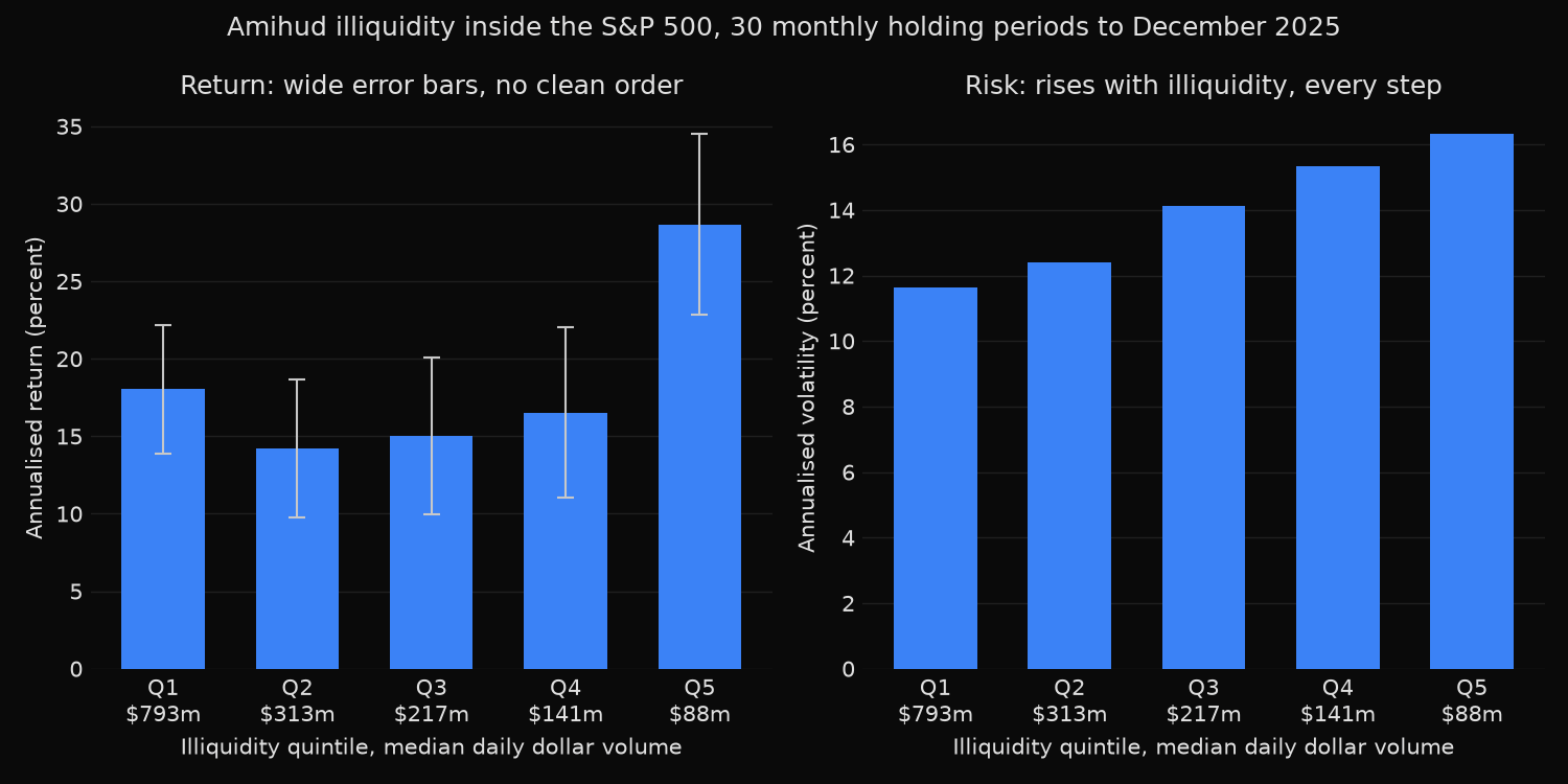
The risk result is clean. Annualised volatility climbs at every single step, from 11.62 percent in the most liquid quintile to 16.32 percent in the least, with a perfect rank correlation across the five groups. Nothing about that ordering is ambiguous. Even inside an index of large companies, the stocks that are harder to trade are the stocks that move around more, and the relationship holds without a single reversal.

The return result looks dramatic and is not trustworthy. The least liquid quintile returned 28.67 percent a year against 18.05 percent for the most liquid, a gap of 9.13 percentage points annualised. That is the sort of number a strategy gets built on. The test says otherwise: t of 1.52, a p-value of 0.141, and a 95 percent confidence interval on the monthly spread running from -0.21 percent to +1.68 percent. Zero sits comfortably inside it. Only 18 of the 30 months were positive, which is barely better than a coin.

The middle of the distribution confirms the doubt. If a genuine premium were being paid for illiquidity, returns would rise step by step the way volatility does. They do not. Quintile 1 at 18.05 percent beats quintile 2 at 14.19 percent, quintile 3 at 15.02 percent and quintile 4 at 16.53 percent. The whole apparent effect lives in the extreme group, which is what a handful of large individual moves looks like rather than a systematic return.

The last line of the output puts a number on the problem. At the effect size and month-to-month noise actually observed, roughly 52 months of data, near four and a half years, would be needed before the spread reached a t-statistic of 2. This study has 30. The honest reading is not that the illiquidity premium is absent inside the S&P 500; it is that 30 months cannot tell the difference between a 9 point premium and nothing at all.

So what?

Do not size a position on the 9 point gap. A confidence interval that spans zero means the strategy could equally be earning nothing, and the non-monotonic middle is the tell that separates a real factor from a lucky tail. Any backtest producing a headline spread should be run through the same two checks before it goes further: does the effect increase monotonically across the sort, and how wide is the interval around it?

The volatility result, by contrast, is solid enough to use. Within a large-cap universe, the Amihud measure is a dependable proxy for how much a position will move, available from daily prices without options data or a risk model. That makes it useful for position sizing and for flagging which index members will be expensive to exit in a stressed market, which is exactly when the measure matters.

For anyone who does want to test the premium properly, the arithmetic above sets the requirement: at least five years of monthly rebalances before the result means anything, and preferably a universe that extends below large caps, where the illiquid tail is genuinely illiquid rather than merely less traded than Apple.

Built with xfinlink — free financial data API for Python. pip install -U xfinlink