

Does Volatility Targeting Improve Sharpe Ratios? Seven-Asset Backtest in Python
July 27, 2026
What's the question?
Volatility clusters. Quiet days tend to follow quiet days and violent days follow violent days, a property of asset returns documented since Mandelbrot studied cotton prices in 1963. Realised volatility over the past month therefore says something about volatility over the next few days, though nothing reliable about direction.
Volatility targeting turns that property into a position-sizing rule: hold an amount inversely proportional to recent realised volatility, so exposure rises when markets are calm and falls when they are turbulent. Moreira and Muir published a version of this in the Journal of Finance in 2017 and reported large Sharpe ratio gains, and volatility scaling is now standard machinery in managed futures and risk premia products.
The narrower question is whether the rule survives mechanical application across asset classes, with the volatility estimate lagged so that nothing measured on a trading day can influence the position held during it.
The approach
Seven exchange-traded funds span US large caps (SPY), US small caps (IWM), developed international equity (EFA), emerging markets (EEM), listed real estate (VNQ), long-dated Treasuries (TLT) and gold (GLD). Daily total returns run from January 2007 to July 2026, covering the 2008 crash, March 2020 and the 2022 rates repricing.
- Measure realised volatility as the standard deviation of the previous 20 daily returns, annualised by the square root of 252.
- Lag it one day, so the position taken on any trading day uses only volatility observable through the prior close.
- Set exposure to a 15% annualised target divided by the lagged estimate, capped at 2.0x. The cap matters: uncapped exposure reached 4.7x in the calm of August 2017.
- Charge one basis point on the notional traded whenever exposure changes.
- Rescale the targeted series by a constant so its full-sample volatility matches buy and hold, making growth and drawdown comparable. Sharpe is unaffected by constant scaling.
- Run it again with the lag removed, as a control on how much a one-day timing error flatters the result.
Step 6 is the part most backtests skip. A rule that sizes today’s position using today’s volatility looks like a strategy and behaves like a forecast of something already known.
Code
import numpy as np
import pandas as pd
import xfinlink as xfl

xfl.set_api_key("YOUR_API_KEY")  # free at https://xfinlink.com/signup

TICKERS = ["SPY", "IWM", "EFA", "EEM", "VNQ", "TLT", "GLD"]
TARGET_VOL, LOOKBACK, MAX_LEVERAGE, COST = 0.15, 20, 2.0, 0.0001

px = pd.concat([xfl.prices(t, start="2006-11-01", fields=["close", "return_daily"])
                for t in TICKERS], ignore_index=True)

def sharpe(r):
    return r.mean() / r.std() * np.sqrt(252)

def backtest(returns, lag):
    """lag=1 uses only information available before the trading day; lag=0 peeks."""
    realised = returns.rolling(LOOKBACK).std() * np.sqrt(252)
    weight = (TARGET_VOL / realised.shift(lag)).clip(upper=MAX_LEVERAGE)
    frame = pd.DataFrame({"r": returns, "w": weight}).dropna()
    frame = frame[frame.index >= "2007-01-01"]
    turnover = frame["w"].diff().abs().fillna(0.0)
    return frame["r"], frame["w"] * frame["r"] - COST * turnover

for t in TICKERS:
    r = px[px["ticker"] == t].sort_values("date").set_index("date")["return_daily"].dropna()
    bh, net = backtest(r, lag=1)
    _, peek = backtest(r, lag=0)
    print(f"{t}: buy-and-hold {sharpe(bh):.2f}  targeted {sharpe(net):.2f}  "
          f"look-ahead {sharpe(peek):.2f}")
Full script with formatting and visualisation: volatility-targeting-sharpe-ratio-backtest-python.py
Output
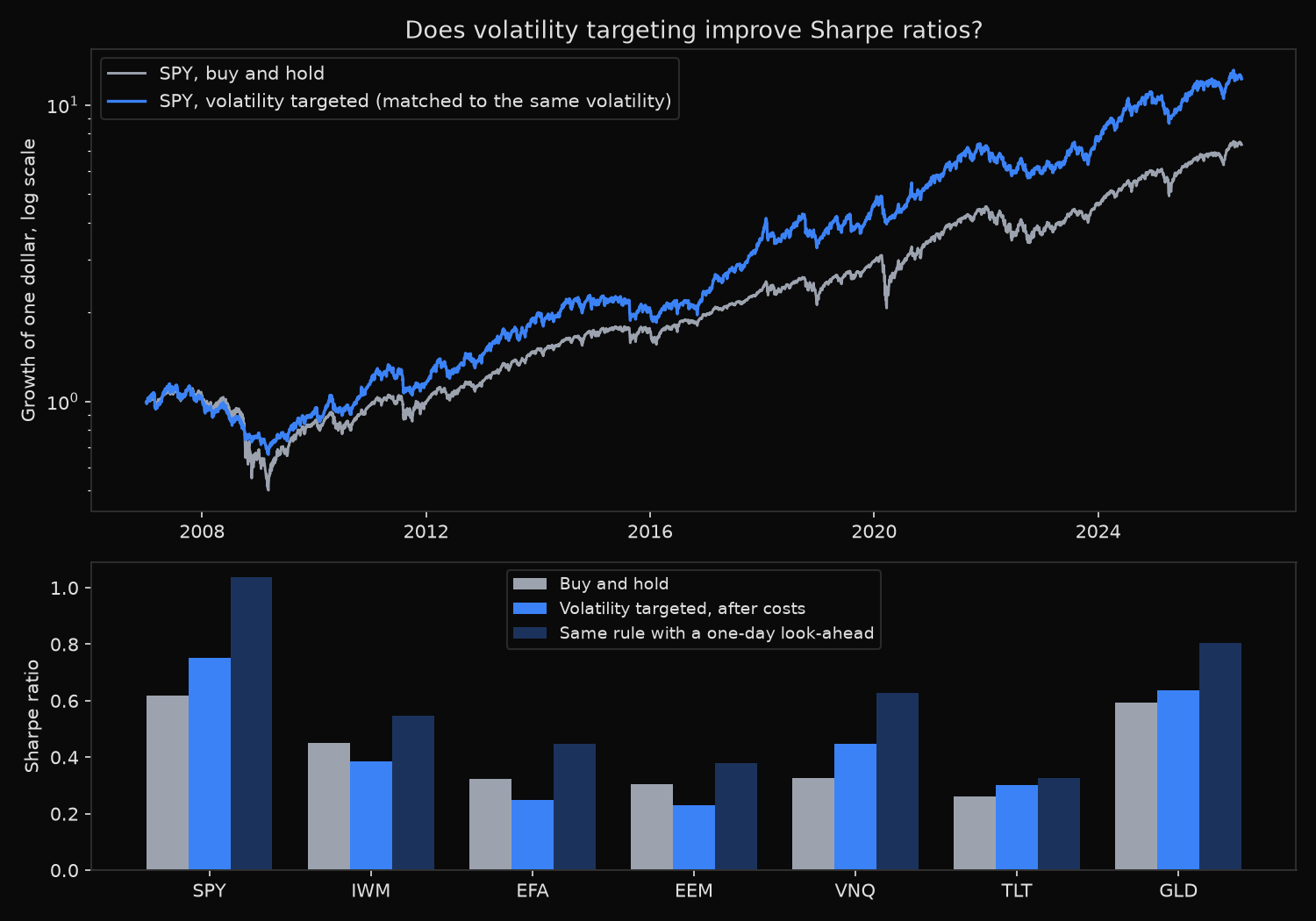
Volatility targeting versus buy and hold, 2007-01-01 to 2026-07-24
20-day realised volatility, 15% annualised target, leverage capped at 2.0x, 1bp per unit traded
Sharpe ratio here is mean return over volatility, no risk-free deduction

Ticker     Days  B&H Sharpe  Targeted  Avg exposure  Turnover
-------------------------------------------------------------
SPY        4920        0.62      0.75          1.18     10.3x
IWM        4920        0.45      0.39          0.84      8.3x
EFA        4920        0.32      0.25          1.05      9.5x
EEM        4920        0.31      0.23          0.82      8.2x
VNQ        4920        0.32      0.45          0.94      8.9x
TLT        4920        0.26      0.30          1.20     10.2x
GLD        4920        0.59      0.64          1.07     10.6x

Volatility-matched comparison (both series rescaled to equal volatility)
Ticker     B&H CAGR  Targeted   B&H MaxDD  Targeted   Ann vol
-------------------------------------------------------------
SPY          10.7%     13.7%      -55.2%    -42.2%     19.6%
IWM           8.4%      6.7%      -59.0%    -45.4%     24.7%
EFA           4.8%      3.1%      -61.0%    -46.9%     21.6%
EEM           4.7%      2.5%      -66.4%    -59.7%     28.0%
VNQ           5.4%      9.2%      -73.1%    -53.8%     29.5%
TLT           2.8%      3.5%      -48.4%    -46.8%     15.0%
GLD           9.5%     10.4%      -45.6%    -57.8%     18.1%

Look-ahead control: same rule, volatility measured through the trading day itself
Ticker    Correct lag  Same-day peek  Inflation
-----------------------------------------------
SPY              0.75           1.04       0.29
IWM              0.39           0.55       0.16
EFA              0.25           0.45       0.20
EEM              0.23           0.38       0.15
VNQ              0.45           0.63       0.18
TLT              0.30           0.33       0.03
GLD              0.64           0.81       0.17

Median Sharpe: buy and hold 0.32, targeted 0.39, targeted with same-day peek 0.55
Median max drawdown: buy and hold -59.0%, targeted -46.9%
Sharpe improved on 4 of 7 assets; drawdown shrank on 6 of 7
What this tells us
Two results point in different directions, and the split is the finding.
Drawdown control works almost everywhere. Six of seven assets took a smaller worst-case loss, and the median maximum drawdown fell from 59.0% to 46.9% at matched volatility. The mechanism is direct: 2008, 2020 and 2022 each began with a volatility spike, so every subsequent leg down arrived with exposure already cut, and SPY exposure averaged 0.30 across September and October 2008. Real estate improved most, from 73.1% to 53.8%.
Return improvement is far less uniform. Sharpe rose on four assets and fell on three: SPY gained most, 0.62 to 0.75, while EEM fell from 0.31 to 0.23. The reason is symmetric to the reason drawdowns improved, because rebounds also arrive during high-volatility periods, and in emerging markets and small caps they were violent enough that being underweight through them cost more than the avoided losses were worth. Gold shows a third pattern, its Sharpe improving while its drawdown got worse: the 45.6% slide that ended in December 2015 was a slow grind at ordinary volatility, which the rule met with average exposure of 1.03.
The look-ahead control prices a single day of hindsight. Median Sharpe jumps from 0.39 to 0.55 once the volatility estimate may include the day being traded, and SPY jumps from 0.75 to 1.04. Nothing changed but the timestamp on one input.
Costs are not the constraint. Annual turnover runs 8.2 to 10.6 times capital, yet at one basis point that removes about one hundredth of a Sharpe point, and at five basis points the median targeted Sharpe still holds at 0.37.
So what?
Treat volatility targeting as a risk-shaping tool rather than a return-improving one. The drawdown evidence holds across six of seven asset classes and three separate crises; the Sharpe evidence does not, and applying the rule to emerging markets or small caps in the expectation of better risk-adjusted returns has the historical record pointing the other way.
The practical order when sizing positions is to decide first whether a smaller worst case is worth surrendering part of the rebound, then apply the rule only where that trade is acceptable. The same four-of-seven split held at lookbacks of 10, 60 and 120 days and at targets of 10% and 20%, so the specific parameters are not doing the work.
For anyone reading someone else’s volatility-scaled backtest, run the lag-zero control first. It takes one changed argument, and it separates a genuine 0.75 from a hindsight-assisted 1.04.
Built with xfinlink — free financial data API for Python. pip install xfinlink
pip install xfinlink