
Does Mean Reversion Survive Trading Costs? Moving-Average Deviations in Python
September 9, 2026
What’s the question?
A stock trading well below its own 50-day average is either cheap or falling for a reason. Mean-reversion rules take the first view: buy the stretch, wait for the price to return to the average, sell. Whether that return trip exists, how long it takes, and whether what arrives beats the cost of trading are three questions; most versions of the rule answer only the first.
The Augmented Dickey-Fuller test (ADF) answers it by looking for a unit root, the signature of a series that wanders with no fixed mean pulling it back; a p-value below 0.05 rejects that and calls the series stationary. Speed is separate: regress today’s deviation from the average on yesterday’s for a coefficient b, and the sessions needed to close half the gap come to -ln(2)/ln(b). That is the half-life.
Cost is the third question, and a trap sits in front of it. Prices fall below their averages mostly when the whole market falls, so the bounce that follows may be the index recovering rather than anything about the stock.
The approach
- Take the S&P 500 as it stood on 2019-12-31 from a point-in-time membership record, carrying each company by entity id so that a recycled ticker cannot substitute one series for another. 501 entities.
- Pull the daily adjusted close for 2020-01-01 to 2024-12-31. The series carries no dividend component, so every return below is a price return.
- Companies without a complete series for the window leave the sample, as do those whose adjusted price moves more than 40% in one session, a size that means a corporate action. 439 remain.
- Take each company’s deviation: log price minus its own trailing 50-session average. Run ADF on the deviation and on the log price, then fit AR(1) for the half-life.
- Scale the deviation by its own trailing 250-session standard deviation. The two windows consume 300 sessions, so signals begin in March 2021.
- Mark a signal wherever the scaled deviation sits at or below -1.5, record the price return over the next 5 sessions, and compare it with that company’s average 5-session return.
- Repeat that comparison after subtracting the equal-weighted return of all 439 companies that date, which strips out the market’s move, then charge 20 basis points (0.20%) for the round trip.
Code
import numpy as np
import pandas as pd
import xfinlink as xfl
from statsmodels.tsa.stattools import adfuller

xfl.set_api_key("YOUR_API_KEY")  # free at https://xfinlink.com/signup

MA, SD, HOLD, ZLIM, COST = 50, 250, 5, -1.5, 0.0020

roster = xfl.index("sp500", as_of="2019-12-31")
ids = sorted({int(e) for e in roster["entity_id"].dropna()})
px = pd.concat([xfl.prices(entity_id=ids[i:i + 20], start="2020-01-01", end="2024-12-31",
                           fields=["adj_close"], max_rows=200000)
                for i in range(0, len(ids), 20)], ignore_index=True)

rows, fwds, sigs = [], {}, {}
for eid, g in px.groupby("entity_id"):
    g = g.sort_values("date").drop_duplicates("date")
    p = np.log(g["adj_close"].to_numpy())
    if len(g) < 1200 or np.max(np.abs(np.diff(p))) > 0.40:
        continue
    s = pd.Series(p, index=g["date"].to_numpy())
    dev = s - s.rolling(MA).mean()                    # log price less its average
    z = dev / dev.rolling(SD).std()
    fwd = np.expm1(s.shift(-HOLD) - s)                # forward 5-session return
    valid = dev.notna() & z.notna() & fwd.notna()
    sig = valid & (z <= ZLIM)
    if int(valid.sum()) < 500 or int(sig.sum()) < 20:
        continue
    d = dev[valid].to_numpy()
    b = np.polyfit(d[:-1], d[1:], 1)[0]               # AR(1) on the deviation
    fwds[eid], sigs[eid] = fwd.where(valid), sig
    rows.append(dict(entity_id=eid, adf_p_dev=adfuller(d, autolag="AIC")[1],
                     adf_p_px=adfuller(s.to_numpy(), autolag="AIC")[1],
                     half_life=-np.log(2) / np.log(b),
                     mu_sig=float(fwd[sig].mean()), mu_all=float(fwd[valid].mean())))

res = pd.DataFrame(rows).set_index("entity_id")
F = pd.DataFrame(fwds)                                # date x company
S = pd.DataFrame(sigs).reindex_like(F).fillna(False).astype(bool)
X = F.sub(F.mean(axis=1), axis=0)                     # less the cross-section that day

res["edge"] = res.mu_sig - res.mu_all
res["mu_sig_x"] = [X[e][S[e]].mean() for e in res.index]
res["edge_x"] = res.mu_sig_x - [X[e][F[e].notna()].mean() for e in res.index]
print(res[["half_life", "edge", "edge_x"]].mean(), (res.edge_x > COST).mean())
Full script with formatting and visualisation: does-mean-reversion-survive-trading-costs-python.py
Output
S&P 500 at 2019-12-31 carried by entity id | priced 2020-01-01 to 2024-12-31
439 companies after screens | 31,208 signals, 2021-03-10 to 2024-12-23 | 419,204 company-days

Augmented Dickey-Fuller, stationary at 5%
  log price                         32 of 439
  deviation from 50-day average    439 of 439

Half-life of a deviation, AR(1), trading sessions
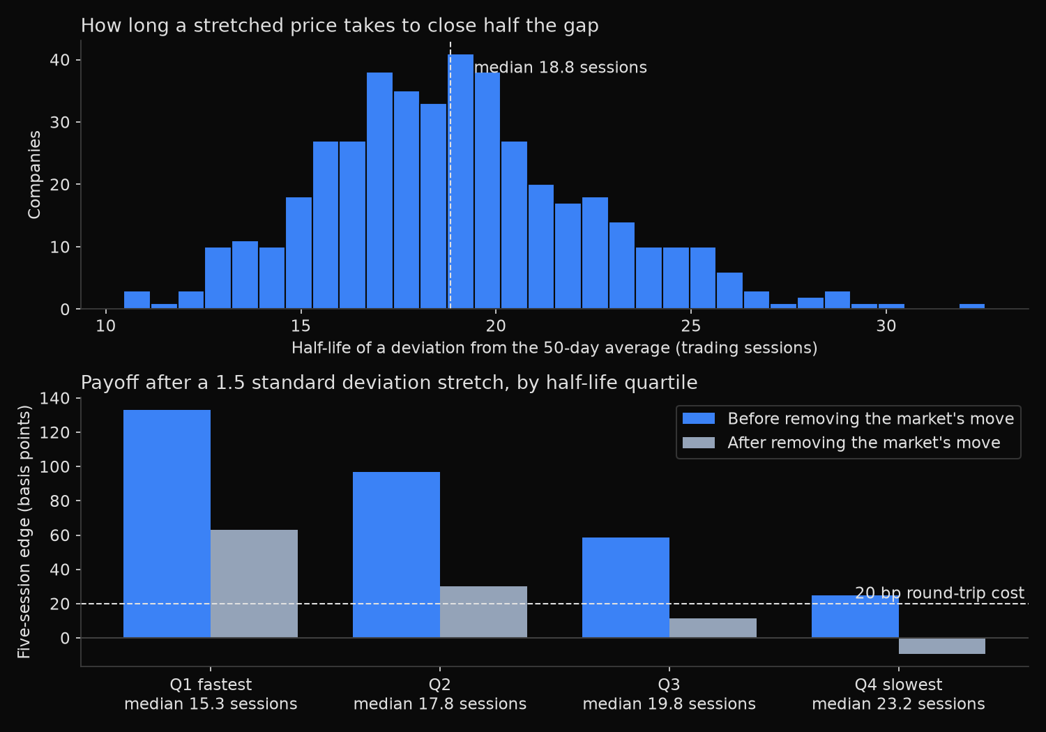
  median 18.8   quartiles 16.7 to 21.1   range 10.5 to 32.5

Forward 5-session price return after the deviation reaches -1.5 sd
  every day, average company               15.8 bp
  after a signal                           94.1 bp
  edge                                     78.3 bp   t 17.00   80.6% of companies positive
  edge less the market's move              23.8 bp   t  6.36   62.0% of companies positive
  same, net of a 20 bp round trip          3.8 bp             51.0% of companies positive

By half-life quartile                    raw edge   less market
  Q1 fastest  110 names, median 15.3     133.0 bp      63.1 bp
  Q2          110 names, median 17.8      96.7 bp      30.1 bp
  Q3          109 names, median 19.8      58.6 bp      11.2 bp
  Q4 slowest  110 names, median 23.2      24.9 bp      -9.4 bp

By signal year                           raw edge   less market
  2021   2,730 signals              142.1 bp      42.6 bp
  2022  16,931 signals               77.0 bp      15.9 bp
  2023   6,455 signals               46.8 bp      -4.1 bp
  2024   5,092 signals               59.7 bp       2.1 bp
What this tells us
The two ADF results split cleanly. Only 32 of 439 log price series reject the unit root at 5%, while the deviation rejects in all 439. That is close to mechanical, since subtracting a trailing average removes the drifting level, and it is a warning: a test passing on 439 of 439 names says nothing about which of them is worth trading. The median company closes half a deviation in 18.8 sessions, quartiles at 16.7 and 21.1, none outside 10.5 to 32.5, so a five-session hold collects about a sixth of the decay.
The raw payoff reads well: 94.1 basis points over five sessions after a signal against 15.8 on an average day, an edge of 78.3 with a t statistic of 17.00, positive in 80.6% of companies. Most of it belongs to the market. Removing the cross-section’s own move on the same dates cuts the edge to 23.8 basis points, and the event count shows why: 16,931 of the 31,208 signals fall in 2022, when index-wide declines pushed most members below their averages at once. The five-session windows overlap, so the t statistics are generous.
A 20 basis point round trip leaves 3.8 basis points for the average company and 51.0% of the sample above water, a coin toss.
Sorting on half-life changes that. The fastest quartile, median 15.3 sessions, keeps 63.1 basis points after the market is removed; the slowest, median 23.2 sessions, gives back 9.4. The rule is identical across the four groups; only the estimated speed of decay differs.
So what?
Estimate the half-life before trading the rule, not after. One regression per name separates a group worth 63 basis points a trade from a group worth less than nothing, and it sets the holding period: five sessions against an 18.8-session half-life leaves most of the reversion uncollected.
Hedge the market leg or accept that most of the payoff is index direction: seven tenths of the raw edge is the S&P 500 recovering, available more cheaply through the index.
Set the cost assumption first, then check what survives it. At 20 basis points only the fastest quartile clears with room, so anyone paying wider, or trading less liquid names, should treat the rule as unprofitable until their own fills prove otherwise.
Built with xfinlink — free financial data API for Python. pip install -U xfinlink
pip install -U xfinlink