Does the Turn-of-the-Month Effect Still Work? Calendar Anomaly Test in Python

What’s the question?

The turn-of-the-month effect is the claim that equity returns concentrate in a narrow window straddling the month boundary: the last trading day of one month together with the first few of the next. Robert Ariel documented the pattern in 1987, and Lakonishok and Smidt confirmed it a year later across ninety years of Dow data. The reported result was striking. In some samples the entire market return accrued during those days, and the rest of the month contributed nothing.

The proposed mechanism is cash flow rather than sentiment. Wages, pension contributions and retirement account deposits arrive on a monthly cycle, index funds put that money to work as it lands, and institutional mandates often rebalance at month end. Buying pressure therefore clusters at a predictable point in the calendar.

A calendar pattern is the easiest kind of anomaly to trade, which is also the reason to doubt that one survives. No forecasting is required, the entry and exit dates are known years ahead, and the capital sits idle for most of the month. If the pattern still paid, it would be unusually simple money.

The approach

Testing this requires an equal-weighted cross-section rather than an index level, so that the answer describes the average company instead of the largest few.

1. Rebuild the S&P 500 roster as it stood at each year end from 2014 to 2024, and count a company on a given date only if it was a member at the previous year end.
2. Pull daily returns for that universe from 2015 through 2025.
3. Average the returns across all member companies on each trading day, giving one equal-weighted return per day.
4. Label each day by its position in the month, counting forward from the first trading day and backward from the last.
5. Compare the classic window, the last trading day plus the first three, against every other day, and test each position separately.

The panel holds 1,360,168 daily observations across 696 companies and 2,766 trading days.

Code

import xfinlink as xfl
import pandas as pd
import numpy as np
from scipy import stats

xfl.set_api_key("YOUR_API_KEY")  # free at https://xfinlink.com/signup

rosters = {y: set(xfl.index("sp500", as_of=f"{y}-12-31")["entity_id"])
           for y in range(2014, 2025)}
universe = sorted(set().union(*rosters.values()))

px = xfl.prices(entity_id=universe, start="2015-01-01", end="2025-12-31",
                fields=["return_daily"], max_rows=500000)
px["date"] = pd.to_datetime(px["date"])

# a company counts only in years it was actually in the index
px["prior_year"] = px["date"].dt.year - 1
px = px[[e in rosters.get(y, set())
         for e, y in zip(px["entity_id"], px["prior_year"])]]

daily = px.groupby("date")["return_daily"].agg(["mean", "size"])
daily = daily[daily["size"] >= 100].rename(columns={"mean": "ret"}).reset_index()

daily["ym"] = daily["date"].dt.to_period("M")
daily["from_start"] = daily.groupby("ym").cumcount() + 1
daily["from_end"] = daily.groupby("ym").cumcount(ascending=False)
daily["tom"] = (daily["from_end"] == 0) | (daily["from_start"] <= 3)

inside, outside = daily[daily["tom"]]["ret"], daily[~daily["tom"]]["ret"]
print(stats.ttest_ind(inside, outside, equal_var=False))

Full script with formatting and visualisation: turn-of-the-month-effect-python.py

Output

panel rows 1,360,168  entities 696
trading days 2766  2015-01-02 to 2025-12-31

turn-of-month days: n=528  mean=+0.0313%
all other days:     n=2238  mean=+0.0520%
difference -0.0208pp  t=-0.39  p=0.700

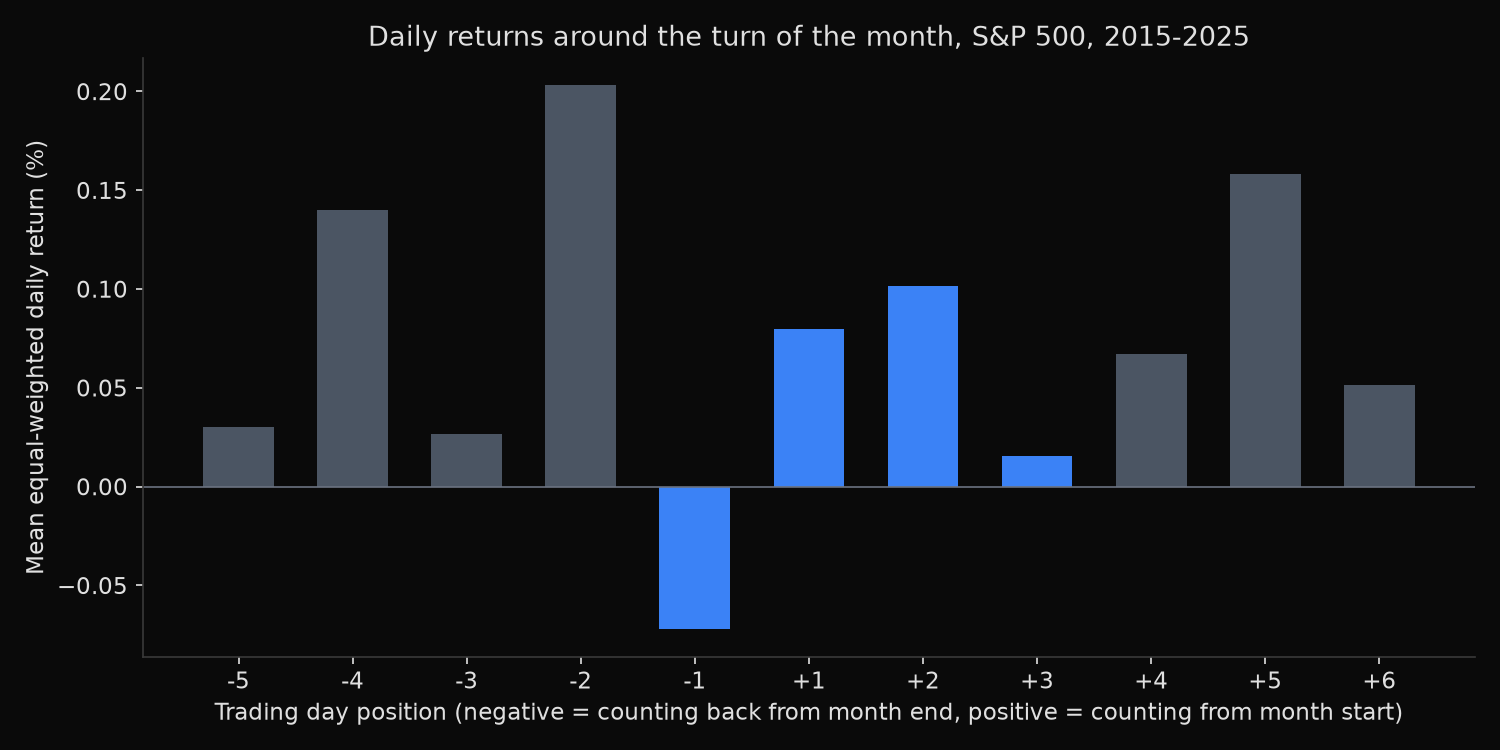
mean return by position in month, tested against every other day:
  -5: n=132  mean=+0.0301%  t=-0.20  p=0.843
  -4: n=132  mean=+0.1401%  t=+0.90  p=0.371
  -3: n=132  mean=+0.0264%  t=-0.23  p=0.818
  -2: n=132  mean=+0.2030%  t=+1.83  p=0.069
  -1: n=132  mean=-0.0722%  t=-1.49  p=0.138
  +1: n=132  mean=+0.0799%  t=+0.33  p=0.738
  +2: n=132  mean=+0.1017%  t=+0.56  p=0.574
  +3: n=132  mean=+0.0156%  t=-0.33  p=0.745
  +4: n=132  mean=+0.0672%  t=+0.18  p=0.861
  +5: n=132  mean=+0.1584%  t=+1.28  p=0.203
  +6: n=132  mean=+0.0514%  t=+0.03  p=0.977

turn-of-month beat the rest of the month in 5 of 11 years

What this tells us

The classic window did not outperform. Turn-of-month days averaged +0.0313% against +0.0520% for every other day, so the window was worse by 0.0208 percentage points, with a t-statistic of −0.39 and a p-value of 0.700. The sign is the opposite of what the anomaly predicts, and the magnitude is indistinguishable from zero. Across the eleven calendar years the window beat the rest of the month five times, which is what a fair coin produces.

The day-by-day profile explains why no window definition rescues the result. The single strongest day in the month is the second-to-last trading day at +0.2030%, which sits outside the classic window entirely. The last trading day, the one the cash-flow story identifies as the strongest candidate, is the only negative position in the table at −0.0722%. A mechanism driven by month-end inflows should produce its largest effect exactly where this sample produces its smallest. A first-trading-day analysis takes the window apart day by day on ETFs over a longer history, with bond funds as a control.

The second-to-last day carries a p-value of 0.069, which looks suggestive in isolation. Eleven positions were tested. Under pure noise, roughly one test in ten clears a 0.10 threshold by chance, so finding one near-significant position among eleven is the expected outcome rather than evidence of anything. Treating it as a discovery is the error that calendar research is most prone to. A bootstrap test of month-by-weekday rules sizes that error when dozens of rules are searched.

None of this means the flows described in the original papers stopped. Wages and pension contributions still arrive monthly. What it means is that the resulting price pressure no longer survives into realised returns at a size worth measuring, which is the normal fate of a documented pattern that requires no skill to exploit.

So what?

A calendar overlay built on the turn of the month has no support in this sample. Holding a large-cap portfolio for four days a month and sitting in cash otherwise would have captured less per day than staying invested, before any consideration of transaction costs, which for a strategy trading twelve times a year would be substantial.

The finding is more useful as a constraint on execution than as a signal. If a mandate already requires trading at month end, this evidence indicates that timing carries no systematic penalty or premium, and the decision can rest on liquidity and tracking error instead of on an expected calendar return. Shifting a backtest’s rebalance day through the month is the experiment in a rebalance-date sweep.

Two extensions would be worth running before the effect is dismissed everywhere. The original studies covered small companies and much longer histories, and the pattern was always strongest in the least liquid names, so a test on a broader universe may reach a different answer. Non-US markets with different payroll and pension calendars are a separate question that this panel does not address.

Built with xfinlink — free financial data API for Python.