
Which Assets Hedge Inflation Shocks? Macro Factor Betas in Python
July 31, 2026
What's the question?
Portfolio risk gets measured against equities far more often than against the economy. A book can be diversified across sectors and still hold one directional bet on the macroeconomy, because two forces move most assets: the pace of real activity, and the rate at which prices rise.
A macro factor beta measures that exposure. It is the slope from regressing an asset’s return on a macro variable, so a beta of 2 means the asset gains 2 percent when the factor rises 1 percent. Official statistics on output and prices are the natural regressors, and the worst available: monthly, late, revised. Markets price the same information continuously, and two spreads between traded funds stand in for the official series:
- Growth: industrial metals minus gold, DBB minus GLD. Both are metals held partly as stores of value, so the difference removes the common currency and real-rate component and leaves industrial demand.
- Inflation: inflation-linked Treasuries minus nominal Treasuries of similar duration, TIP minus IEF. The difference tracks breakeven inflation, the rate at which holding either bond pays the same.
Which assets load positively on each, and have those answers held still?
The approach
Fifteen liquid funds cover US large and small cap equity, developed and emerging international equity, seven US sectors, listed real estate, long Treasuries and corporate credit. None appears in either factor spread.
- Pull daily total returns from January 2015 to July 2026 and compound them into weekly returns ending Friday, leaving 602 observations.
- Build the two factor series as return differences between the funds named above.
- Regress each asset’s weekly return on both factors jointly, with Newey-West standard errors at four lags so volatility clustering does not inflate the t-statistics.
- Refit on 2015 to 2020 and on 2021 to 2026, splitting where US inflation moved from below target to well above it.
Fitting both together matters: metals rally in an expansion and so do breakevens, and at a correlation of +0.19 a single-factor regression would credit one with part of the other’s effect.
Code
import pandas as pd
import statsmodels.api as sm
import xfinlink as xfl

xfl.set_api_key("YOUR_API_KEY")  # free at https://xfinlink.com/signup

FACTOR_LEGS = ["DBB", "GLD", "TIP", "IEF"]
ASSETS = ["SPY", "IWM", "EFA", "EEM", "XLE", "XLF", "XLI", "XLK",
          "XLP", "XLU", "XLY", "VNQ", "TLT", "LQD", "HYG"]

px = pd.concat(
    [xfl.prices(t, start="2015-01-01", fields=["return_daily"]) for t in FACTOR_LEGS + ASSETS]
)
daily = px.pivot_table(index="date", columns="ticker", values="return_daily")

# keep weeks with complete daily coverage across every series
obs = daily.notna().resample("W-FRI").sum()
complete = obs.eq(obs.max(axis=1), axis=0).all(axis=1)
weekly = ((1 + daily.fillna(0)).resample("W-FRI").prod() - 1)[complete].iloc[1:]

growth = weekly["DBB"] - weekly["GLD"]
inflation = weekly["TIP"] - weekly["IEF"]
X = sm.add_constant(pd.DataFrame({"growth": growth, "inflation": inflation}))

for a in ASSETS:
    m = sm.OLS(weekly[a], X).fit(cov_type="HAC", cov_kwds={"maxlags": 4})
    print(f"{a}  growth {m.params['growth']:+.3f} (t {m.tvalues['growth']:.1f})  "
          f"inflation {m.params['inflation']:+.3f} (t {m.tvalues['inflation']:.1f})  "
          f"R2 {m.rsquared:.2f}")
Full script with formatting and visualisation: macro-factor-betas-growth-inflation-python.py
Output
Sample: 2015-01-09 to 2026-07-31  (602 weeks)
Growth factor    DBB-GLD   annualised vol  20.4%
Inflation factor TIP-IEF   annualised vol   4.1%
Factor correlation: +0.19

                         growth beta      t   inflation beta      t     R2
XLE   Energy                   0.230    3.8            3.238    6.5   0.27
XLF   Financials               0.248    5.8            1.801    4.7   0.21
IWM   US small cap             0.190    3.5            1.764    3.5   0.16
XLI   Industrials              0.179    4.0            1.684    3.9   0.18
SPY   S&P 500                  0.144    4.0            1.213    3.6   0.14
XLY   Discretionary            0.178    3.8            1.168    2.8   0.10
EFA   Developed ex-US          0.138    2.9            1.151    2.5   0.12
XLK   Technology               0.192    4.4            1.045    3.2   0.09
EEM   Emerging markets         0.216    4.8            0.972    2.7   0.11
VNQ   REITs                   -0.002   -0.0            0.747    1.5   0.02
XLU   Utilities               -0.125   -2.2            0.634    1.3   0.03
XLP   Staples                 -0.013   -0.4            0.590    2.0   0.03
HYG   High yield               0.038    1.6            0.425    1.6   0.05
LQD   IG credit               -0.052   -1.3           -0.203   -0.5   0.02
TLT   Long Treasuries         -0.150   -2.5           -1.429   -3.6   0.26

2015-2020: 312 weeks   inflation factor vol  3.8%   corr(SPY, inflation factor) +0.55
2021-2026: 290 weeks   inflation factor vol  4.4%   corr(SPY, inflation factor) +0.12

                                growth beta           inflation beta
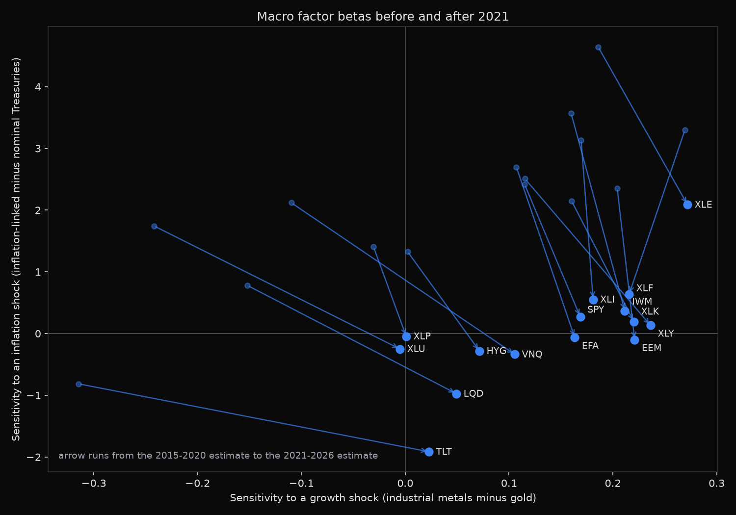
                       2015-2020  2021-2026    2015-2020   2021-2026    change
XLE   Energy                0.19       0.27         4.64        2.09     -2.56
XLF   Financials            0.27       0.22         3.30        0.64     -2.66
IWM   US small cap          0.16       0.21         3.57        0.37     -3.20
XLI   Industrials           0.17       0.18         3.14        0.55     -2.58
SPY   S&P 500               0.12       0.17         2.42        0.27     -2.14
XLY   Discretionary         0.12       0.24         2.51        0.13     -2.38
EFA   Developed ex-US       0.11       0.16         2.70       -0.06     -2.76
XLK   Technology            0.16       0.22         2.15        0.19     -1.95
EEM   Emerging markets      0.20       0.22         2.35       -0.10     -2.45
VNQ   REITs                -0.11       0.11         2.12       -0.34     -2.46
XLU   Utilities            -0.24      -0.01         1.74       -0.25     -1.99
XLP   Staples              -0.03       0.00         1.41       -0.04     -1.45
HYG   High yield            0.00       0.07         1.33       -0.28     -1.61
LQD   IG credit            -0.15       0.05         0.78       -0.97     -1.75
TLT   Long Treasuries      -0.31       0.02        -0.82       -1.91     -1.10
What this tells us
The growth column sorts assets the way a business cycle textbook would. Financials at 0.248 and energy at 0.230 head the list, technology and industrials sit in the middle, and the two negative loadings that clear significance belong to utilities at -0.125 and long Treasuries at -0.150. Regulated revenue does not expand with industrial demand, and a fixed coupon loses value when activity accelerates.
The inflation column reads differently. Thirteen of the fifteen loadings are positive. Energy is the outlier at 3.238 with a t-statistic of 6.5, close to triple the S&P 500 reading of 1.213, and long Treasuries at -1.429 provide the only significant negative.
That average hides two different worlds. Splitting the sample moves every inflation beta down, by 1.10 for long Treasuries and by 3.20 for small caps, and the S&P 500 falls from 2.42 to 0.27. Eight assets end the second period with a negative loading, seven of which were positive in the first. Before 2020, US inflation ran below the Federal Reserve’s target, so rising breakevens signalled recovering demand and equities read the news as good; after 2021 the same signal meant tightening. The collapse is not a scaling artefact, because the factor was slightly more volatile in the second period, 4.4 percent against 3.8 percent annualised, while its correlation with S&P 500 returns fell from 0.55 to 0.12.
Two exposures survived the break: energy kept an inflation beta of 2.09, and long Treasuries stayed negative at -1.91. A one standard deviation weekly move in the inflation factor is about 0.57 percent, so energy’s full-sample loading is roughly 1.8 percent of return per shock, against 0.7 percent for the S&P 500 and 0.15 percent on the post-2021 estimate. R-squared runs from 0.02 to 0.27, about what two macro factors should explain in weekly returns.
So what?
Portfolio macro beta is the weighted sum of the holdings’ betas. A 60/40 book of SPY and TLT carries an inflation beta of -0.60 on the post-2021 estimates, 0.6 times 0.27 plus 0.4 times -1.91, so both legs lose in an inflation shock. 2022 delivered exactly that.
Where to close the gap is arithmetic rather than preference. The bond leg supplies -0.76 of the -0.60 on its own, so holding that 40 percent in cash rather than in long Treasuries would put the total at +0.16 without touching a single equity position. Buying energy instead is expensive: funding a beta of 2.09 out of an equity leg at 0.27 takes about a third of the portfolio to reach zero, which is the practical reason inflation hedging usually happens on the bond side.
These loadings changed sign inside eleven years, so a table computed once and reused is a hazard. Re-estimate on a rolling two to three year window, watch the equity block’s inflation beta, and treat any hedge whose sign depends on the pre-2021 sample as unproven.
Built with xfinlink — free financial data API for Python. pip install -U xfinlink
pip install -U xfinlink