Which Sectors Actually Drive "Sell in May"? Sector Seasonality Analysis in Python

September 8, 2026

What’s the question?

"Sell in May and go away" is the claim that shares earn almost all of their return in the six months from November to April and almost nothing from May to October. Sven Bouman and Ben Jacobsen put numbers on it across 37 markets in a 2002 American Economic Review paper, and it remains one of the few calendar anomalies still argued about.

Almost every test measures it on an index: one series, one average for the whole market. That summary cannot say whether the seasonal is spread across the market or concentrated in a corner of it, and the two possibilities call for different trades. A gap present in every sector is a property of equities. A gap carried by cyclicals is a sector tilt wearing calendar clothing, and harvesting it means rotating between sectors rather than moving in and out of the market.

The approach

A sector answer needs an equal-weighted cross-section rather than an index level, so it describes the average member of a sector, not its largest company.

1. Rebuild the S&P 500 roster as it stood on 1 January of each year from 2001 through 2024, and count a company in a given year only while it was a member that year.
2. Pull monthly total returns for that universe, requested by entity id rather than by ticker, so a symbol later reassigned to a different company cannot splice two histories into one series.
3. Winsorise each monthly cross-section at its 1st and 99th percentiles. Lehman Brothers fell 99.2 percent in September 2008 and American International Group rose 245 percent in August 2009; uncapped, single observations like those set a sector average by themselves.
4. Average the capped returns across members within each sector, then label each month November-April or May-October.
5. Compare the two seasons with a Welch t-test, which does not assume the halves share a variance, and multiply mean monthly returns by six so the figures read as six-month returns.

The panel holds 135,111 company-months across 914 companies and 288 calendar months, with 431 to 499 index members in any given month. Real Estate reaches five members only in 2006, so it contributes 228 months. Companies without a complete monthly series or a sector classification for the window leave the sample.

Code

import numpy as np
import pandas as pd
import xfinlink as xfl
from scipy import stats

xfl.set_api_key("YOUR_API_KEY")  # free at https://xfinlink.com/signup

WINTER = {11, 12, 1, 2, 3, 4}

rosters = {y: sorted(set(xfl.index("sp500", as_of=f"{y}-01-01", limit=1000)
                         ["entity_id"].dropna().astype(int)))
           for y in range(2001, 2025)}
universe = sorted(set().union(*[set(v) for v in rosters.values()]))

chunks = [universe[i:i + 25] for i in range(0, len(universe), 25)]
px = pd.concat([xfl.prices(entity_id=c, start="2001-01-01", end="2024-12-31",
                           interval="1mo", fields=["return_daily"],
                           max_rows=300000) for c in chunks], ignore_index=True)

px["date"] = pd.to_datetime(px["date"])
px["year"] = px["date"].dt.year
px["month"] = px["date"].dt.to_period("M")

memb = pd.DataFrame([(y, e) for y, ids in rosters.items() for e in ids],
                    columns=["year", "entity_id"])
panel = (px.merge(memb, on=["year", "entity_id"], how="inner")
         .dropna(subset=["return_daily", "gics_sector"]))

lo = panel.groupby("month")["return_daily"].transform(lambda s: s.quantile(0.01))
hi = panel.groupby("month")["return_daily"].transform(lambda s: s.quantile(0.99))
panel["ret"] = panel["return_daily"].clip(lo, hi)

sm = (panel.groupby(["gics_sector", "month"])
      .agg(ret=("ret", "mean"), n=("entity_id", "nunique")).reset_index())
sm = sm[sm["n"] >= 5]
sm["season"] = np.where(sm["month"].dt.month.isin(WINTER), "winter", "summer")

for sector, g in sm.groupby("gics_sector"):
    w = g.loc[g["season"] == "winter", "ret"]
    s = g.loc[g["season"] == "summer", "ret"]
    t, p = stats.ttest_ind(w, s, equal_var=False)
    print(f"{sector:<24}{600 * w.mean():>8.2f}%{600 * s.mean():>8.2f}%"
          f"{600 * (w.mean() - s.mean()):>7.2f}{t:>7.2f}{p:>8.3f}")

Full script with formatting and visualisation: sell-in-may-by-sector-python.py

Output

point-in-time universe: 978 entities
panel: 135,111 company-months, 914 companies, 288 months

Sector                    Nov-Apr  May-Oct     Gap      t       p   mths
------------------------------------------------------------------------
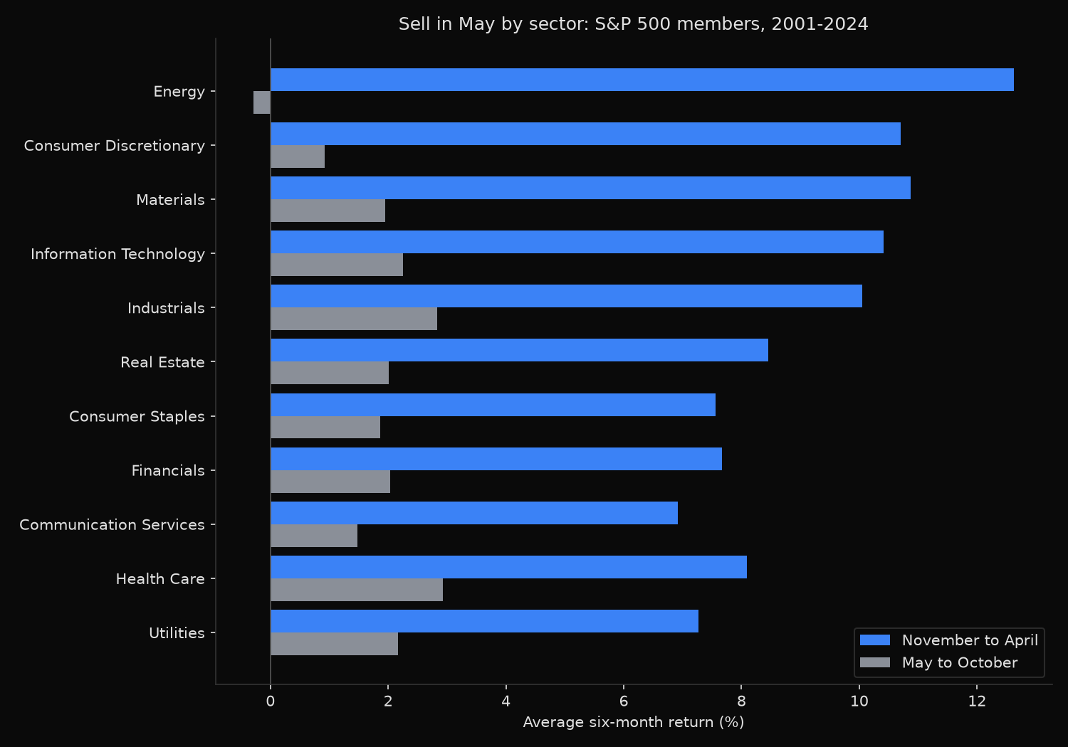
Energy                     12.63%   -0.29%  12.91   2.14   0.033    288
Consumer Discretionary     10.70%    0.92%   9.78   2.11   0.036    288
Materials                  10.87%    1.95%   8.92   2.20   0.028    288
Information Technology     10.41%    2.25%   8.16   1.54   0.124    288
Industrials                10.05%    2.83%   7.22   1.83   0.069    288
Real Estate                 8.45%    2.01%   6.44   1.16   0.246    228
Consumer Staples            7.57%    1.87%   5.70   2.31   0.021    288
Financials                  7.66%    2.03%   5.63   1.31   0.190    288
Communication Services      6.92%    1.47%   5.45   1.37   0.173    288
Health Care                 8.10%    2.93%   5.16   1.70   0.090    288
Utilities                   7.27%    2.17%   5.10   1.60   0.110    288
------------------------------------------------------------------------
All members, equal weight    9.10%    1.79%   7.31   2.03   0.043    288

What this tells us

Direction is unanimous and size is not. All eleven sectors earned more between November and April than between May and October, and the gap runs from 5.10 percentage points in Utilities to 12.91 in Energy, a spread of two and a half times. Energy is the extreme case in both halves: its winter average of 12.63 percent is the highest in the table, and its summer average of minus 0.29 percent means 24 years of May-to-October holds produced slightly less than nothing.

The ranking follows economic sensitivity rather than anything about the calendar. Energy, Materials and Consumer Discretionary sit at the top, Utilities and Health Care at the bottom, the standard cyclical-versus-defensive ordering. Defensive sectors sell what people buy in every month of the year, leaving less of a seasonal cycle for a calendar rule to catch.

Statistical reliability does not follow the size of the gap. Consumer Staples has one of the smaller gaps at 5.70 points and the lowest p-value at 0.021, because its month-to-month variation is small enough that a modest difference stands out; Energy has more than twice the gap and reaches only 0.033. Five of the eleven sectors sit above 0.10. The market-wide equal-weighted gap of 7.31 points does clear the conventional 5 percent bar at 0.043, though eleven positive sector gaps are not eleven independent confirmations, since sector returns move together.

So what?

The version of "sell in May" most people picture is holding the market from November and sitting in cash from May. That trade survives the test at the equal-weighted market level, and it remains the weaker way to act on the result: it stakes everything on one 7.31-point estimate and forfeits an average of 1.79 percent every summer sitting out.

A tilt uses the same evidence better. The winter premium is two and a half times larger in Energy than in Utilities, so overweighting Energy and Materials from November and rotating into Utilities and Health Care in May takes the part of the pattern with an economic story behind it while staying invested throughout. Two rebalances a year make transaction costs a rounding error against gaps of this size.

Size that tilt against the evidence rather than the headline. The widest gaps sit in the most volatile sectors, which is why Energy’s 12.91 points carries a smaller t-statistic than Consumer Staples’ 5.70, and 24 winters is a short sample for a signal that fires twice a year. Re-run the split on the sector and window that match the mandate before committing capital.