
What’s the question?
Standard deviation treats an upside surprise and a downside surprise as equally bad. For an investor deciding how much to fear a crash, that is the wrong assumption, because the two are not equally bad at all. Skewness is the statistic that separates them.
Skewness measures the asymmetry of a return distribution. A positive value means the right tail is longer: the occasional move is a large gain. A negative value means the left tail is longer, and the rare large move is a loss. A symmetric distribution, including the normal distribution that sits inside most risk models, has a skewness of zero. Real returns are rarely symmetric, and whether the asymmetry points up or down decides whether the surprises in a series tend to help or hurt. Kurtosis, the measure of how heavy the tails are, gets a separate treatment in a test for fat tails.
The question here has a specific target. Individual stocks and the index built from them are usually assumed to share the same shape. If they do not, and if the market is skewed differently from its own components, then diversification is changing the character of the risk rather than only its size.
The approach
The sample pairs the market, represented by SPY, with sixteen of its larger members across sectors. The window runs from 2016 to August 2026, and its length is deliberate. Skewness is driven by rare, large moves, so a short and calm stretch produces an unstable estimate that can carry the wrong sign; a decade that contains the 2020 crash and the 2022 bear market gives the tails enough observations to settle.
For each series the analysis computes the skewness of daily returns, then compounds the daily returns into monthly returns and computes the skewness again. Comparing the index against its components at both horizons is the whole test.
Code
import pandas as pd
from scipy.stats import skew
import xfinlink as xfl

xfl.set_api_key("YOUR_API_KEY")  # free at https://xfinlink.com/signup

tickers = ["SPY", "AAPL", "MSFT", "NVDA", "AMZN", "GOOGL", "JPM", "JNJ",
           "XOM", "PG", "KO", "HD", "WMT", "UNH", "V", "CVX", "CAT"]

px = xfl.prices(tickers, start="2016-01-01", end="2026-08-21",
                fields=["return_daily"])
px["date"] = pd.to_datetime(px["date"])

rows = []
for t in tickers:
    sub = px[px["ticker"] == t][["date", "return_daily"]].dropna()
    monthly = sub.set_index("date")["return_daily"].add(1).resample("ME").prod().sub(1)
    rows.append({"ticker": t,
                 "daily_skew": skew(sub["return_daily"]),
                 "monthly_skew": skew(monthly.dropna())})

d = pd.DataFrame(rows)
print(d.sort_values("daily_skew").to_string(index=False))
Full script with formatting and visualisation: stock-return-skewness-python.py
Output
ticker  daily_skew  monthly_skew
   UNH      -1.332         0.249
    HD      -0.751        -0.083
    KO      -0.553        -0.547
   SPY      -0.313        -0.418
   CVX      -0.309         0.418
   JNJ      -0.192         0.040
   CAT      -0.017         0.113
   XOM      -0.008         0.265
 GOOGL       0.036         0.312
  AAPL       0.111        -0.049
    PG       0.161        -0.100
     V       0.201        -0.021
   WMT       0.216        -0.369
  MSFT       0.272         0.140
   JPM       0.306        -0.146
  AMZN       0.316         0.273
  NVDA       0.510        -0.029

SPY daily skew:   -0.313   monthly skew: -0.418
single stocks, median daily skew: 0.073, mean: -0.065
stocks less negatively skewed than SPY (daily):   13 of 16
stocks less negatively skewed than SPY (monthly): 15 of 16
What this tells us
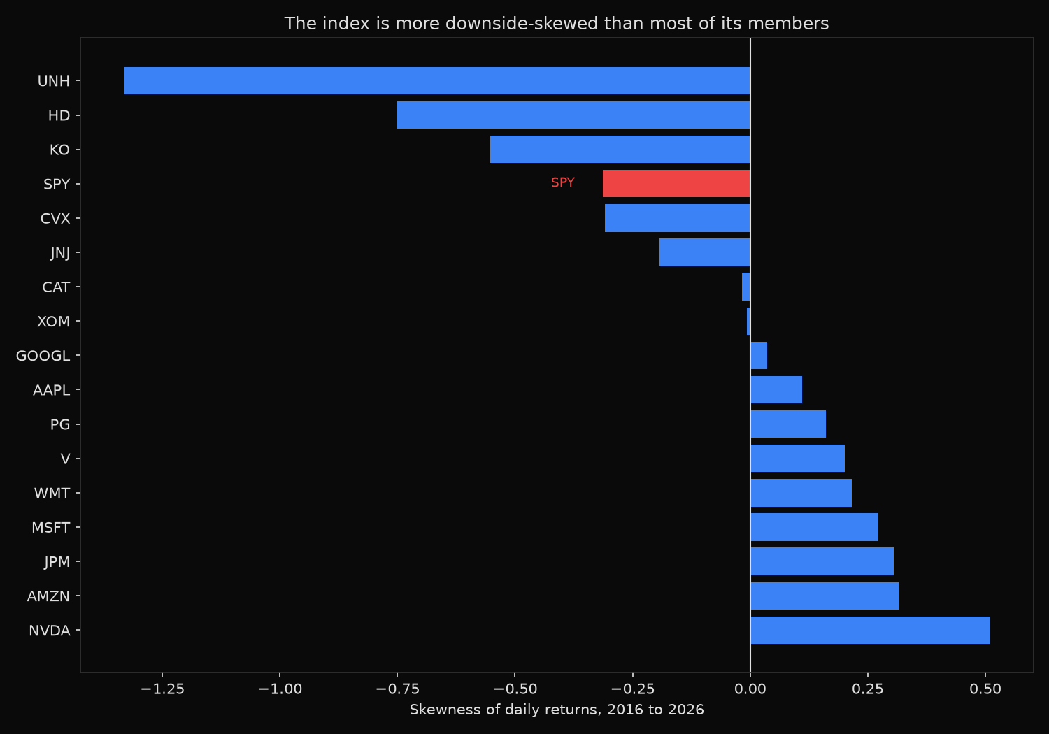
The index is negatively skewed at both horizons: SPY comes in at negative 0.31 on daily returns and negative 0.42 on monthly returns. Its distribution carries a fatter left tail, and the fattening grows as the horizon lengthens. The large moves in the market are, on balance, the moves down.
Individual stocks behave differently. The median single-stock daily skew is a positive 0.07, and thirteen of the sixteen members are less negatively skewed than the index. At the monthly horizon the gap widens to fifteen of sixteen. The mean single-stock skew is slightly negative at negative 0.065, but that figure is pulled down almost entirely by one name, so the median is the honest summary.
The reason sits in what drives each kind of move. A single company jumps on its own news: an earnings beat, a drug trial, a bid to buy it. Those idiosyncratic surprises arrive up about as often as down, which keeps a single stock near zero or tilted positive. A crash is the opposite kind of event, the one thing that strikes every holding at once. Averaging across many names cancels the private jumps while leaving the shared decline untouched, so the portfolio keeps the left tail and loses the right. UnitedHealth is the exception that confirms the mechanism: its daily skew of negative 1.33 is the most negative in the group, produced not by any market crash but by a company-specific collapse in 2025. Such events can drive one name sharply negative, yet they do it one name at a time, which is exactly why they wash out in aggregate while systematic crashes accumulate.
So what?
Diversification lowers volatility, and it concentrates negative skew at the same time. The index an investor diversifies into is more asymmetric to the downside than the average stock diversified out of. That is a consequence of correlation, not a defect in the index, and it has direct consequences for how a portfolio should be protected and measured.
A risk model that assumes normal returns will misjudge the two cases in opposite directions: roughly right about a single volatile stock, too optimistic about the left tail of a diversified index. Value-at-risk and volatility targeting both inherit that blind spot. It is also why the standard crash hedge is written on the index rather than on single names, since the index is where the downside asymmetry actually lives.
For construction the lesson is sharper. Adding more equity names does little to soften a drawdown, because it does nothing to the shared risk that produces the negative skew. Cutting the equity weight, or adding an asset whose bad months do not line up with stocks’, is what changes the shape. Volatility tells you how large the swings are; skewness tells you which side to guard, and for a stock portfolio the answer is the downside.
Built with xfinlink — free financial data API for Python.