Can 2x Leveraged Sector ETFs Beat Their Sector? Volatility Drag Analysis in Python

September 12, 2026

What’s the question?

Every 2x leveraged sector fund carries a toll that the sector itself does not. The fund restores a fixed leverage ratio at each close, which forces it to sell after losses and buy after gains, and that repeated adjustment costs return in any market that oscillates. The toll has a closed form: for a fund targeting L times the daily return of an index whose daily returns have variance σ², the annual gap between the fund’s log growth and L times the index’s log growth is approximately (L² − L)σ²/2, which at L = 2 collapses to σ² on its own.

That fact is usually presented as a warning. Read the other way, it is a selection rule. Doubling a sector is worth doing only when the sector compounds faster than the toll it charges, and both quantities are measurable in advance. A sector at 27% volatility is charging around 7.5 points a year before fees, while one at 14% is charging under 2.

The practical question, then, is which sectors compound fast enough to pay their own toll, and whether fifteen years of live fund returns behave the way the formula says.

The approach

Nine ProShares Ultra funds each target twice the daily return of a United States sector index. Each is paired with the Select Sector SPDR covering the same sector: ROM against XLK for technology, DIG against XLE for energy, and so on across financials, industrials, materials, health care, utilities, staples, and consumer discretionary.

1. Pull daily total returns, price change plus distributions, for all eighteen funds from 2010-01-04 to 2024-12-31, keeping the 3,774 dates on which every series trades.
2. Compound each series in logs. The benchmark for a 2x fund is twice the sector’s cumulative log growth, which is what an investor who borrowed once at the start and never rebalanced would have earned.
3. Measure the reset cost from the sector’s own return path alone: compound twice each daily return, then subtract that from twice the compounded sector return.
4. Compare the measured cost against σ², the closed-form prediction.
5. Attribute whatever remains of each fund’s shortfall to fees, financing, and imperfect tracking, with the realised daily multiple against the Select Sector partner reported as a check.
6. Compare each sector’s own annual log growth against its total shortfall. The 2x fund beats the sector when growth exceeds shortfall, and loses when it does not.

Code

import numpy as np
import pandas as pd
import xfinlink as xfl

xfl.set_api_key("YOUR_API_KEY")  # free at https://xfinlink.com/signup

PAIRS = {"XLB": "UYM", "XLE": "DIG", "XLF": "UYG", "XLI": "UXI", "XLK": "ROM",
         "XLP": "UGE", "XLU": "UPW", "XLV": "RXL", "XLY": "UCC"}
NAME = {"XLB": "Materials", "XLE": "Energy", "XLF": "Financials",
        "XLI": "Industrials", "XLK": "Technology", "XLP": "Staples",
        "XLU": "Utilities", "XLV": "Health Care", "XLY": "Discretionary"}

px = xfl.prices(list(PAIRS) + list(PAIRS.values()), start="2010-01-04",
                end="2024-12-31", fields=["return_daily"], max_rows=200000)
r = px.pivot(index="date", columns="ticker", values="return_daily").dropna()
years = len(r) / 252.0

rows = []
for sec, lev in PAIRS.items():
    ru, rl = r[sec], r[lev]
    g_sec = np.log1p(ru).sum()                 # sector, buy and hold
    g_lev = np.log1p(rl).sum()                 # the live 2x fund
    g_reset = np.log1p(2 * ru).sum()           # costless daily-reset 2x
    rows.append({
        "sector": NAME[sec], "fund": lev,
        "vol": ru.std(ddof=1) * np.sqrt(252),
        "mult": np.polyfit(ru, rl, 1)[0],      # realised daily multiple
        "sec_x": np.exp(g_sec), "lev_x": np.exp(g_lev), "tgt_x": np.exp(2 * g_sec),
        "shortfall": (2 * g_sec - g_lev) / years,
        "drag": (2 * g_sec - g_reset) / years,
        "sigma2": ru.var(ddof=1) * 252,
    })
t = pd.DataFrame(rows).sort_values("vol", ascending=False).reset_index(drop=True)
t["cost"] = t["shortfall"] - t["drag"]
t["growth"] = np.log(t["sec_x"]) / years        # sector log growth per year
t["beat"] = t["growth"] > t["shortfall"]        # 2x fund ahead of the sector

print(f"{len(r)} trading days, {years:.1f} years, 2010-01-04 to 2024-12-31
")
print(f"{'Sector':<14}{'Fund':<6}{'Vol':>6}{'Mult':>6}{'Sector':>9}"
      f"{'Fund':>9}{'Target':>10}{'Short':>8}{'Drag':>8}{'Sig2':>7}{'Cost':>7}")
for _, x in t.iterrows():
    print(f"{x.sector:<14}{x['fund']:<6}{x.vol:>5.1%}{x['mult']:>6.2f}"
          f"{x.sec_x:>8.2f}x{x.lev_x:>8.2f}x{x.tgt_x:>9.2f}x"
          f"{x.shortfall:>8.2%}{x.drag:>8.2%}{x.sigma2:>7.2%}{x.cost:>7.2%}")
print(f"
Drag vs sigma^2: mean gap {(t.drag - t.sigma2).mean():>+.3%}, "
      f"correlation {np.corrcoef(t.drag, t.sigma2)[0, 1]:.4f}")
print(f"Cost after drag: {t.cost.min():.2%} to {t.cost.max():.2%}, "
      f"median {t.cost.median():.2%}
")

print("Break-even: the sector must compound faster than the shortfall")
print(f"{'Sector':<14}{'Growth':>8}{'Hurdle':>9}{'Margin':>9}  Fund beat sector")
for _, x in t.sort_values("growth", ascending=False).iterrows():
    print(f"{x.sector:<14}{x.growth:>8.2%}{x.shortfall:>9.2%}"
          f"{x.growth - x.shortfall:>+9.2%}  {'yes' if x.beat else 'no'}")
print(f"{t.beat.sum()} of {len(t)} funds beat their sector over the window")

Full script with formatting and visualisation: leveraged-sector-etf-volatility-drag-python.py

Output

3774 trading days, 15.0 years, 2010-01-04 to 2024-12-31

Sector        Fund     Vol  Mult   Sector     Fund    Target   Short    Drag   Sig2   Cost
Energy        DIG   27.4%  1.94    2.46x    1.04x     6.06x  11.74%   7.76%  7.53%  3.98%
Financials    UYG   22.1%  1.82    5.43x   10.56x    29.44x   6.84%   4.97%  4.90%  1.87%
Technology    ROM   21.3%  2.05   12.49x   42.89x   156.02x   8.62%   4.59%  4.53%  4.04%
Materials     UYM   20.9%  2.07    3.53x    3.21x    12.43x   9.05%   4.41%  4.36%  4.64%
Discretionary UCC   20.1%  1.66    9.09x   25.05x    82.60x   7.97%   4.10%  4.02%  3.87%
Industrials   UXI   19.5%  1.90    6.32x   14.69x    39.88x   6.67%   3.83%  3.78%  2.83%
Utilities     UPW   17.6%  1.87    4.12x    7.23x    16.95x   5.69%   3.11%  3.09%  2.58%
Health Care   RXL   16.1%  1.98    5.71x   15.02x    32.63x   5.18%   2.61%  2.59%  2.57%
Staples       UGE   13.7%  1.84    4.44x    9.41x    19.75x   4.95%   1.90%  1.88%  3.06%

Drag vs sigma^2: mean gap +0.066%, correlation 0.9999
Cost after drag: 1.87% to 4.64%, median 3.06%

Break-even: the sector must compound faster than the shortfall
Sector          Growth   Hurdle   Margin  Fund beat sector
Technology      16.86%    8.62%   +8.24%  yes
Discretionary   14.74%    7.97%   +6.77%  yes
Industrials     12.31%    6.67%   +5.64%  yes
Health Care     11.64%    5.18%   +6.45%  yes
Financials      11.29%    6.84%   +4.45%  yes
Staples          9.96%    4.95%   +5.01%  yes
Utilities        9.45%    5.69%   +3.76%  yes
Materials        8.41%    9.05%   -0.64%  no
Energy           6.02%   11.74%   -5.72%  no
7 of 9 funds beat their sector over the window

What this tells us

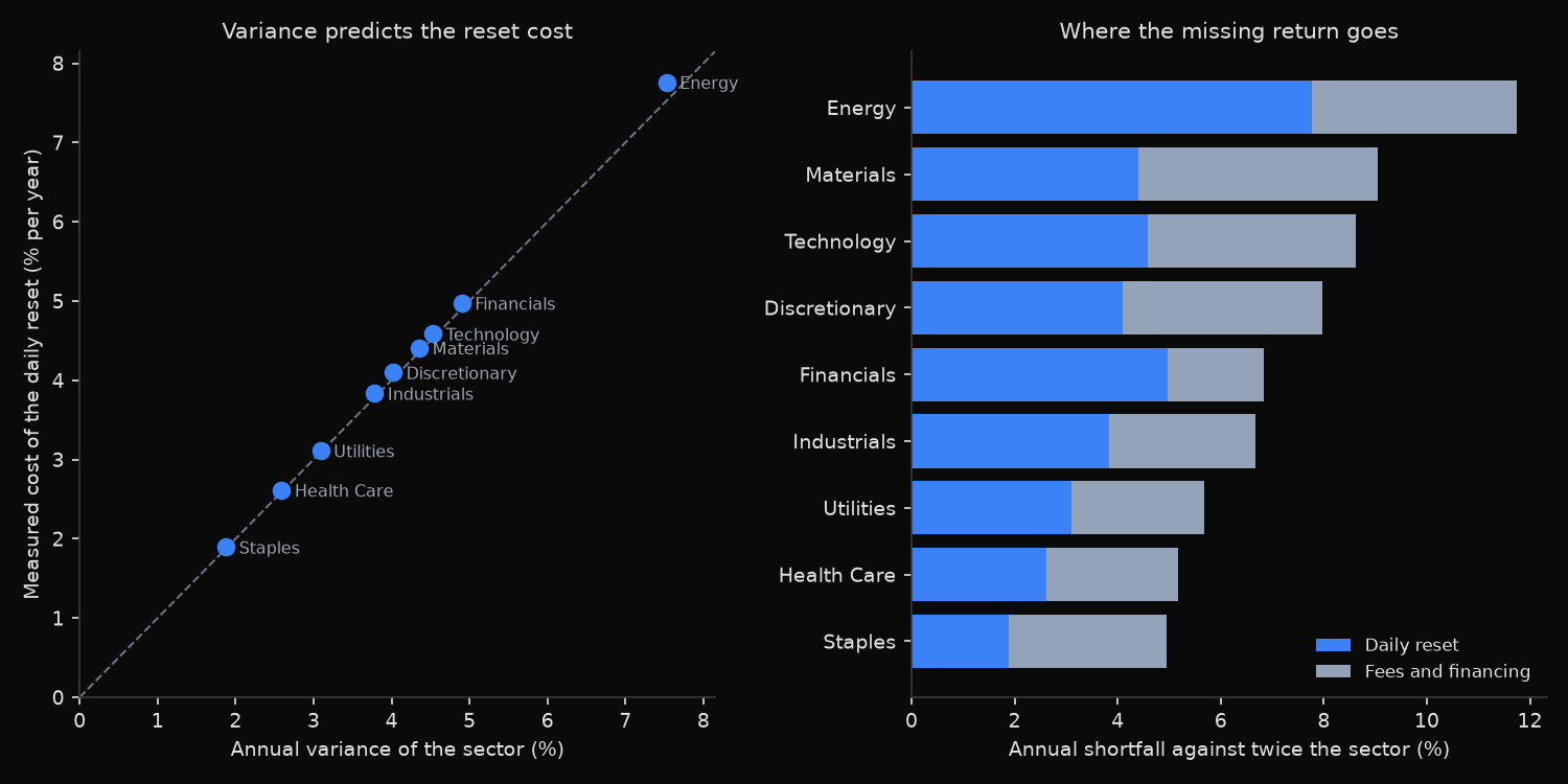
The closed form is close to exact. The measured reset cost sits an average of 0.066 percentage points above σ² across the nine sectors, with a correlation of 0.9999. Staples, calmest at 13.7% volatility, gives up 1.90% a year; energy, at 27.4%, gives up 7.76%. Doubling volatility roughly quadruples the cost, which is what a squared term does.

What remains after the reset cost runs from 1.87% a year for financials to 4.64% for materials, median 3.06%. Published expense ratios of 0.95% account for under a third of that. Financing the borrowed half at short-term rates covers most of the rest, and the realised multiples, spread between 1.66 and 2.07, show the Select Sector SPDR is not a perfect stand-in for every fund’s own benchmark.

Seven of the nine funds still beat their sector outright, which cuts against the usual warning. Technology cleared its 8.62% hurdle by 8.24 points a year and ROM multiplied capital nearly 43 times against XLK’s 12.49, while health care cleared a 5.18% hurdle by 6.45 points. Materials missed by 0.64 points and UYM ended below XLB; energy missed by 5.72 points and DIG turned one dollar into 1.04 while XLE rose 146%.

Energy failed for the reason the formula predicts, carrying the highest volatility in the group alongside the lowest growth. High volatility is not itself disqualifying: financials ran at 22.1% and cleared its hurdle by 4.45 points.

So what?

The selection rule is arithmetic, not judgement. Take the sector’s annualised variance, add roughly 3 percentage points for fees and financing, and that is the compounded annual return the sector must clear for the 2x fund to be worth owning instead of the sector. A 30% volatility sector needs about 12% a year, which few sectors sustain across a full cycle. A 14% volatility sector needs about 5%, which most equity sectors clear comfortably.

Note which side of the calculation is easier to forecast. Volatility persists and can be estimated from recent data, so the hurdle is close to knowable, whereas sector growth over the next decade is not. That asymmetry argues for demanding a wide margin, since materials missed by less than a point and still left its holders behind the plain sector fund.

For a position held today, compute the current hurdle rather than the historical one. Volatility regimes move, and a sector that paid its toll comfortably through a calm decade will charge substantially more in a turbulent one.

Built with xfinlink — free financial data API for Python. pip install -U xfinlink