Does Trading Volume Predict Tomorrow's Volatility? Out-of-Sample Test in Python

August 30, 2026

What’s the question?

Volatility is the number nobody observes and everybody needs. Position sizes, stop distances and margin all rest on an estimate of the next move’s size, and the standard estimate looks backward: an average of recent absolute returns.

The mixture-of-distributions hypothesis, set out by Peter Clark in 1973 and refined by Tauchen and Pitts in 1983, points to a second input. Its claim is that price changes and trading volume are both driven by one hidden variable, the rate at which new information reaches the market: when a lot of news lands, a lot of shares change hands and the price travels a long way. If that is right, today’s volume says something about tomorrow’s move that yesterday’s price changes do not already say.

Same-day co-movement is useless, since by then the move has happened. The test that matters is whether adding volume to a volatility forecast beats one built from past returns alone.

The approach

Two nested regressions per name, then a split-sample forecast.

1. Universe: the S&P 500 as of 2 January 2019, carried by entity_id rather than ticker, so a recycled symbol cannot splice two companies into one series. Daily data runs to 31 December 2025.
2. Volatility predictor: the mean absolute return over the trailing 21 sessions, known at tonight’s close.
3. Volume predictor: log volume minus its own 60-session average. Share counts differ by orders of magnitude across names and drift over time, so detrending in logs is what makes the reading comparable. A value of 0.69 means volume ran at twice its norm.
4. Target: tomorrow’s absolute return. Standard errors are Newey-West with five lags, since absolute returns are strongly autocorrelated.
5. Out-of-sample check: fit both models on 2019-2022, forecast 2023-2025, and score each against the average absolute return of the fitting period. An R-squared above zero beats that constant.

Sessions without a traded volume are excluded, as are names quoted below one dollar and sessions with an absolute return above 50 percent. Names carrying volume on fewer than 95 percent of sessions, or with fewer than 1,200 usable observations, do not enter. That leaves 460 names and 778,518 name-days across all eleven GICS sectors.

Code

import numpy as np
import pandas as pd
import statsmodels.api as sm
import xfinlink as xfl

xfl.set_api_key("YOUR_API_KEY")  # free at https://xfinlink.com/signup

VOL_WIN, TREND_WIN, MIN_OBS = 21, 60, 1200
SPLIT = pd.Timestamp("2023-01-01")

roster = xfl.index("sp500", as_of="2019-01-02")
ids = sorted(roster["entity_id"].dropna().astype(int).unique().tolist())

px = pd.concat(
    [xfl.prices(entity_id=ids[i:i + 50], start="2019-01-01", end="2025-12-31",
                fields=["close", "volume", "return_daily"], max_rows=200000)
     for i in range(0, len(ids), 50)],
    ignore_index=True,
)
px["date"] = pd.to_datetime(px["date"])

rows = []
for eid, g in px.groupby("entity_id"):
    g = g.sort_values("date")
    if (g["volume"].fillna(0) > 0).mean() < 0.95 or g["close"].median() < 1:
        continue
    g = g[(g["volume"] > 0) & g["return_daily"].notna()
          & (g["return_daily"].abs() <= 0.5)]
    if len(g) < MIN_OBS:
        continue
    a, lv = g["return_daily"].abs(), np.log(g["volume"])
    d = pd.DataFrame({
        "date": g["date"].values,
        "y": a.shift(-1).values,                            # tomorrow's absolute return
        "vol": a.rolling(VOL_WIN).mean().values,            # trailing 21-session mean |return|
        "dv": (lv - lv.rolling(TREND_WIN).mean()).values,   # log volume less its 60-session average
    }).dropna()
    if len(d) < MIN_OBS:
        continue

    y = d["y"].to_numpy()
    X0 = sm.add_constant(d[["vol"]].to_numpy())         # volatility only
    X1 = sm.add_constant(d[["vol", "dv"]].to_numpy())   # volatility plus volume
    m0 = sm.OLS(y, X0).fit()
    m1 = sm.OLS(y, X1).fit(cov_type="HAC", cov_kwds={"maxlags": 5})

    tr, te = (d["date"] < SPLIT).to_numpy(), (d["date"] >= SPLIT).to_numpy()
    f0, f1 = sm.OLS(y[tr], X0[tr]).fit(), sm.OLS(y[tr], X1[tr]).fit()
    sst = ((y[te] - y[tr].mean()) ** 2).sum()
    rows.append({
        "t_dv": m1.tvalues[2], "r2_vol": m0.rsquared, "r2_both": m1.rsquared,
        "oos_vol": 1 - ((y[te] - f0.predict(X0[te])) ** 2).sum() / sst,
        "oos_both": 1 - ((y[te] - f1.predict(X1[te])) ** 2).sum() / sst,
    })

R = pd.DataFrame(rows)
R["oos_gain"] = R["oos_both"] - R["oos_vol"]
print(f"names {len(R)}  median t {R['t_dv'].median():.2f}  "
      f"significant {(R['t_dv'] > 1.96).sum()}")
print(f"in-sample R2 {R['r2_vol'].median():.4f} -> {R['r2_both'].median():.4f}")
print(f"out-of-sample R2 {R['oos_vol'].median():.4f} -> {R['oos_both'].median():.4f}  "
      f"improved {(R['oos_gain'] > 0).sum()}")

Full script with formatting and visualisation: does-volume-predict-volatility-python.py

Output

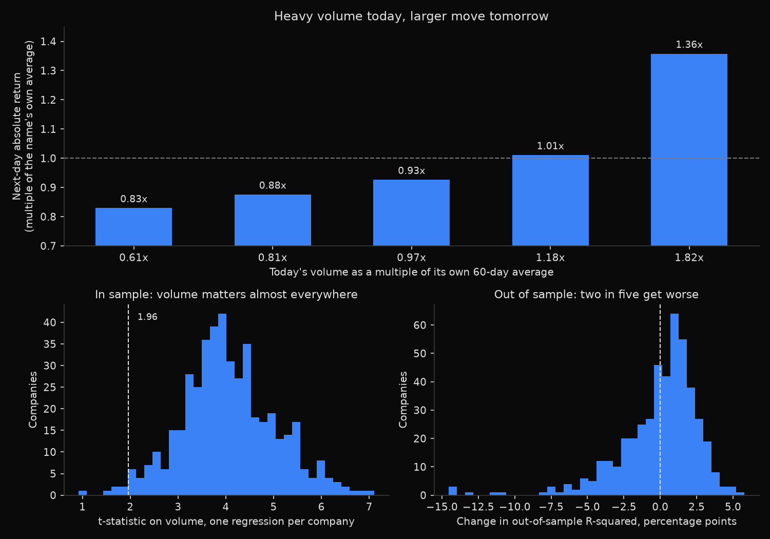
460 names, 778,518 name-days, 2019-03-28 to 2025-12-30

Next-day absolute return by quintile of today's detrended volume
 quintile  volume vs own 60-day avg  next-day |return|   name-days
        1                     0.61x              0.83x     155,714
        2                     0.81x              0.88x     155,698
        3                     0.97x              0.93x     155,696
        4                     1.18x              1.01x     155,698
        5                     1.82x              1.36x     155,712

Per-name regression of tomorrow's |return| on trailing volatility and volume
median t-statistic on detrended volume            3.98
  range of that t-statistic                       0.92 to 7.10
names with t above +1.96                           454 of 460
names with a negative volume coefficient             0 of 460
median R-squared, volatility only               0.1094
median R-squared, volatility plus volume        0.1284
median effect of a doubling in volume             0.37 pp
  against a mean absolute return of               1.39 pp

Out-of-sample: coefficients fitted 2019-2022, tested 2023-2025
median R-squared, volatility only               0.0614
median R-squared, volatility plus volume        0.0675
median change in R-squared                      0.0056
mean change in R-squared                       -0.0006
names improved by adding volume                    275 of 460
names worse by more than 1 R-squared point         127 of 460

What this tells us

The raw relationship runs the way the theory predicts, and it is monotonic. The quietest fifth of a name’s sessions trades at 0.61 times its 60-day norm and is followed by absolute returns of 0.83 times that name’s average; the busiest fifth trades at 1.82 times and is followed by 1.36 times.

Controlling for recent volatility does not remove it. All 460 names carry a positive volume coefficient, 454 clear a Newey-West t-statistic of 1.96, and the median t is 3.98. A doubling of volume adds 0.37 percentage points to the median name’s expected next-day absolute return, against an average of 1.39 percent: a lift of about a quarter. Median in-sample R-squared rises from 10.94 percent to 12.84 percent.

Out of sample the picture is far more sober. Coefficients fitted on 2019-2022 and applied to 2023-2025 raise median R-squared from 6.14 percent to 6.75 percent, a median gain of 0.56 points, against the 1.90 points the median moved in sample. Only 275 of 460 names improve, 127 lose more than a full R-squared point, and the mean change is negative at −0.06 points: the losers lose more than the winners win.

Heavy-volume days are also large-move days, so the two predictors overlap, and in sample the estimator prices that overlap exactly. Out of sample it cannot. Mean absolute returns ran 1.63 percent across 2019-2022 against 1.30 percent across 2023-2025, so a coefficient calibrated through March 2020 is too large for what followed.

So what?

Volume belongs in a volatility forecast as a small correction, not a second engine. The rule that survives the split sample is comparative: a name trading at roughly twice its recent norm should be treated as about 25 percent more volatile tomorrow than its 21-session history alone implies. For a volatility-targeted book that is a real change in size.

The estimation lesson is worth more than the signal. An effect significant on 454 of 460 names improved out-of-sample accuracy for only 275, so per-name t-statistics are the wrong test for a forecasting variable. Shrink the fitted coefficient toward the cross-sectional median, fit over a window spanning calm and stressed markets, and re-fit on a rolling basis.

Run the split-sample step before trusting any new volatility predictor. The median in-sample R-squared moved 1.90 points here against a median out-of-sample gain of 0.56; that ratio, not the t-statistic, is what a position size should be built on.

Built with xfinlink — free financial data API for Python. pip install -U xfinlink