
Does Free Cash Flow Coverage Predict Dividend Cuts Better Than the Payout Ratio? Point-in-Time Screening in Python
September 8, 2026
What’s the question?
The earnings payout ratio divides cash dividends by reported net income. Near 100 percent, the company is handing back everything it earned, and the standard reading is that the dividend is exposed. Almost every stock screener carries the number.
Net income is an accounting result. It absorbs depreciation and impairment charges that move no cash, and it ignores the capital spending needed to keep the business running. Dividends are paid in cash. That gives a second measure: free cash flow coverage, which divides operating cash flow minus capital expenditures by the cash actually distributed to common shareholders. Coverage of 2.0x means the company generated twice what it paid out.
If the two rank companies the same way, the choice between them is cosmetic. If coverage catches dividends that look comfortable on earnings, a screen built on the payout ratio alone leaves risk on the table.
The approach
This needs a period in which a large number of dividends were genuinely cut. The eighteen months after mid-2019 supply one.
- Take the S&P 500 roster as it stood on 28 June 2019, point-in-time and carried by entity id, so a ticker later reassigned cannot substitute one company for another. Names that left the index during the window stay in; those whose listing ended inside it were bought rather than stressed, and leave.
- Keep the regular payers: at least four ex-dividend dates in the preceding twelve months, and a closed fiscal year reporting positive cash dividends to common shareholders. That leaves 382 of the 501.
- Read both ratios from the last fiscal year ending on or before 31 December 2018, each filed months before the formation date, so nothing in the screen depends on information that arrived later.
- Follow the declared dividend per share from ex-dividend records through 31 December 2020, dividing out any split that lands after an ex-date so the series sits on one basis. A cut is a payment below 90 percent of the pre-formation median, or a gap longer than 1.75 normal payment intervals. The median rather than the mean, because one special dividend would raise the bar for everything after it.
The earnings flag fires when the payout ratio exceeds 80 percent or the company lost money; the cash flow flag when coverage falls below 1.0x.
Code
import pandas as pd
import xfinlink as xfl

xfl.set_api_key("YOUR_API_KEY")  # free at https://xfinlink.com/signup

FORM, BASE_START, WIN_END = (pd.Timestamp("2019-06-28"), pd.Timestamp("2018-06-29"),
                             pd.Timestamp("2020-12-31"))

def pull(fn, ids, size, **kw):
    return pd.concat([fn(entity_id=ids[i:i + size], **kw)
                      for i in range(0, len(ids), size)], ignore_index=True)


roster = xfl.index("sp500", as_of="2019-06-28")
ids = sorted(roster["entity_id"].dropna().astype(int).unique())

# fiscal years closed and filed well before the formation date
fund = pull(xfl.fundamentals, ids, 40, period_type="annual", start="2017-06-01",
            end="2018-12-31", fields=["net_income", "free_cash_flow",
                                      "dividends_paid_common"])
fund = fund.sort_values(["entity_id", "period_end"]).groupby("entity_id", as_index=False).tail(1)
payers = fund[fund["dividends_paid_common"] > 0]

px = pull(xfl.prices, payers["entity_id"].astype(int).tolist(), 6, start="2018-06-01",
          end="2020-12-31", fields=["dividend", "split_ratio"])

# a declared dividend is stated in the shares of its day, so divide out later splits
px = px.sort_values(["entity_id", "date"])
px["sr"] = pd.to_numeric(px["split_ratio"], errors="coerce").fillna(1.0)
px["fwd"] = px.groupby("entity_id")["sr"].transform(
    lambda s: s[::-1].cumprod()[::-1].shift(-1).fillna(1.0))
px["div"] = pd.to_numeric(px["dividend"], errors="coerce") / px["fwd"]

# a listing that ends inside the window belongs to a company that was bought
alive = px.groupby("entity_id")["date"].max()
px = px[px["entity_id"].isin(alive[alive >= WIN_END - pd.Timedelta(days=15)].index)]

rows = []
for eid, g in px[px["div"] > 0].groupby("entity_id"):
    g = g.sort_values("date")
    base = g[(g["date"] > BASE_START) & (g["date"] <= FORM)]
    if len(base) < 4:
        continue
    rate = base["div"].median()
    gap = base["date"].diff().dt.days.dropna().median()
    post = g[(g["date"] > FORM) & (g["date"] <= WIN_END)]
    seq = pd.concat([base["date"].tail(1), post["date"], pd.Series([WIN_END])])
    rows.append({"entity_id": eid,
                 "cut": bool((post["div"] < 0.90 * rate).any())
                        or bool(seq.diff().dt.days.max() > 1.75 * gap)})

df = payers.merge(pd.DataFrame(rows), on="entity_id")
df = df[df["net_income"].notna() & df["free_cash_flow"].notna()]
df["payout"] = df["dividends_paid_common"] / df["net_income"]
df["cover"] = df["free_cash_flow"] / df["dividends_paid_common"]
df["earn_flag"] = (df["net_income"] <= 0) | (df["payout"] > 0.80)
df["cash_flag"] = df["cover"] < 1.0

for label, m in [("earnings flag", df.earn_flag), ("cash flow flag", df.cash_flag),
                 ("both", df.earn_flag & df.cash_flag),
                 ("neither", ~df.earn_flag & ~df.cash_flag)]:
    print(f"{label:15s} n={m.sum():3d}  cut rate {df[m].cut.mean() * 100:.1f}%")
Full script with formatting and visualisation: fcf-coverage-vs-payout-ratio-dividend-cuts-python.py
Output
====================================================================================
DIVIDEND CUTS: EARNINGS PAYOUT RATIO VERSUS FREE CASH FLOW COVERAGE
====================================================================================
Roster     S&P 500 as at 2019-06-28, carried by entity id: 501 companies
Sample     382 of them were paying a regular dividend at that date and
           had a closed fiscal year on file
Predictors last fiscal year ending on or before 2018-12-31, so every
           figure was public six months before the window opens
Outcome    a cut is a per-share payment below 90% of the pre-formation
           median, or a gap of more than 1.75 normal payment intervals,
           between 2019-06-28 and 2020-12-31

Cuts in the window: 69 of 382 companies (18.1%)  |  outright reductions 35, skipped payments 41

Each screen on its own
  screen                      flagged  cut rate  not flagged  cut rate
  Earnings payout above 80%        85     28.2%          297     15.2%
  FCF coverage below 1.0x          58     29.3%          324     16.0%

The two screens crossed
                                companies   cuts  cut rate
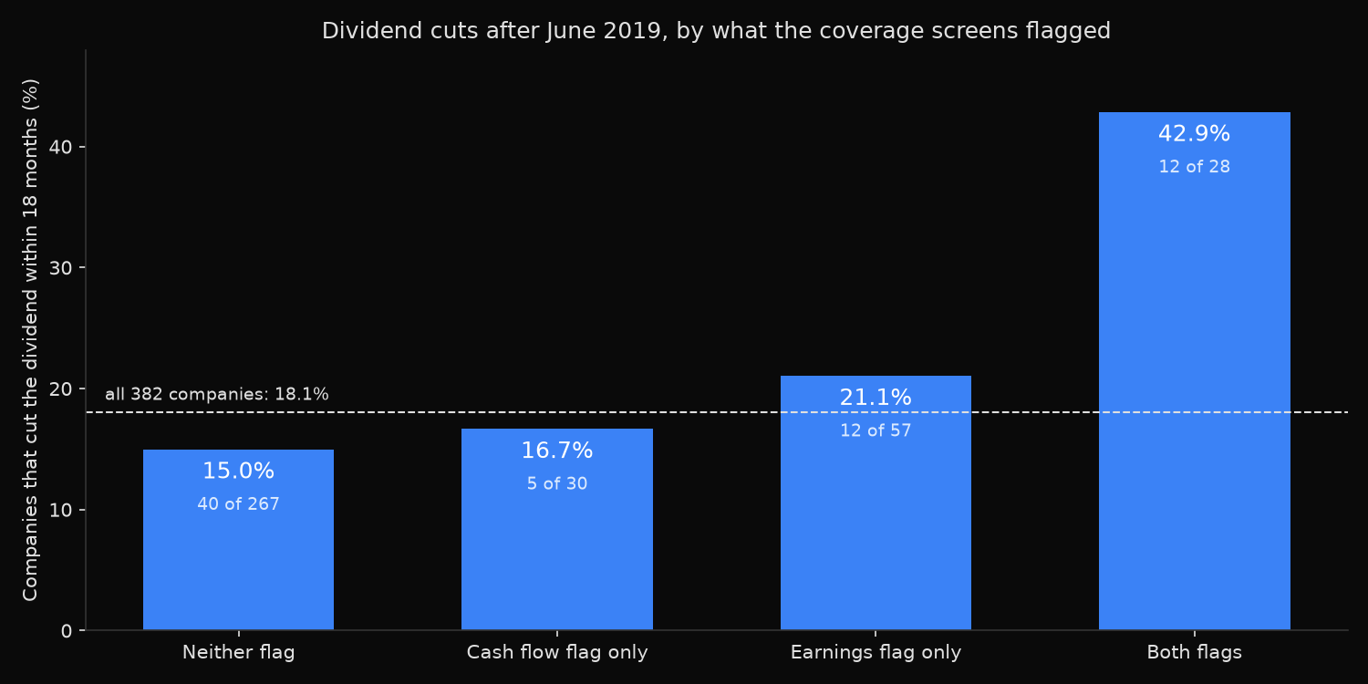
  Neither flag                        267     40     15.0%
  Cash flow flag only                  30      5     16.7%
  Earnings flag only                   57     12     21.1%
  Both flags                           28     12     42.9%
  Both flags against neither, Fisher exact p = 0.00089

Cut rate by free cash flow coverage of the dividend
  bucket               n   cuts     rate
  negative FCF        27      7    25.9%
  0.0 to 1.0x         31     10    32.3%
  1.0 to 1.5x         36     10    27.8%
  1.5 to 2.5x         92     13    14.1%
  above 2.5x         196     29    14.8%

Cut rate by earnings payout ratio
  bucket               n   cuts     rate
  loss-making         18      6    33.3%
  0 to 40%           182     27    14.8%
  40 to 60%           73     14    19.2%
  60 to 80%           42      4     9.5%
  above 80%           67     18    26.9%

By sector
  sector                      n  cuts     rate  med cover  med payout
  Consumer Discretionary     46    24    52.2%      2.74x         42%
  Energy                     23     8    34.8%      1.98x         34%
  Real Estate                28     9    32.1%      1.17x        124%
  Communication Services      6     1    16.7%      1.73x         47%
  Industrials                59     9    15.3%      2.28x         34%
  Materials                  24     3    12.5%      2.57x         32%
  Consumer Staples           34     4    11.8%      2.03x         42%
  Utilities                  25     2     8.0%     -0.26x         62%
  Financials                 68     5     7.4%      4.69x         27%
  Health Care                33     2     6.1%      3.34x         36%
  Information Technology     36     2     5.6%      3.67x         31%

Cuts that neither screen flagged: 40 of 69 (58.0%)
Consumer Discretionary names clean on both screens: 37, of which 18 cut (48.6%)
====================================================================================
What this tells us
One at a time, the two ratios are interchangeable. The payout screen flags 85 companies and 28.2 percent of them cut, against 15.2 percent of the 297 it passed; the coverage screen flags 58 and 29.3 percent of them cut, against 16.0 percent of the rest. Both lift the 18.1 percent base rate by about the same amount.
Crossing them changes the picture. Among the 30 flagged only on cash flow, 16.7 percent cut, indistinguishable from the 15.0 percent recorded by the 267 that neither screen touched. The earnings flag alone reaches 21.1 percent. Where both fire, 12 of 28 companies cut, a rate of 42.9 percent and nearly three times the clean cell, with a Fisher exact p-value of 0.00089. Each ratio alone largely reproduces the other; the added information sits in their agreement.
The sector table shows why. Utilities post a median coverage of negative 0.26x, since a regulated asset base is expanded with borrowed money rather than retained cash, yet only 8.0 percent of them cut. Real estate shows a median payout of 124 percent, since depreciation on buildings pushes net income far below rental cash flow, and 32.1 percent of them cut. Alone, either ratio mostly identifies the accounting shape of an industry. Together, they isolate companies stretched on a basis their own conventions cannot explain away.
A harder result sits underneath. Of the 69 cuts, 40 came from companies neither screen flagged, clustered in consumer discretionary: 37 names there passed both tests and 18 cut anyway, 48.6 percent against a median coverage of 2.74x. Airlines, hotels and cruise operators entered 2020 with well-funded dividends and then lost their revenue.
So what?
Run both ratios and act where they agree. The intersection is 28 names out of 382, tight enough to justify position-level work on each one: the debt maturity schedule, the covenant headroom, the size of the holding. A single flag earns a watch list entry and little more, since a company failing only the coverage test cut at 16.7 percent, no worse than the average payer.
Do not read a clean coverage ratio as safety. Coverage measures whether a dividend survives an ordinary year, not whether it survives a shuttered hotel, and the second scenario drove most of the cuts here. Pair the ratio work with an explicit view on revenue exposure: the sector spread in this window, 52.2 percent for consumer discretionary against 5.6 percent for information technology, was wider than anything the coverage buckets produced.
Build the screen as a joint filter rather than a ranked composite. Averaging two ratios into one score dilutes the very thing that made them useful, which was the requirement that both agree.
Built with xfinlink — free financial data API for Python. pip install -U xfinlink
pip install -U xfinlink