Are Earnings Harder to Forecast Than Revenue? Quarterly Time-Series Models in Python

September 12, 2026

What’s the question?

Almost every company model starts with a quarterly number carried forward from the year-ago quarter. That default has a name in time-series work: the seasonal random walk, which treats last year’s same quarter as the best available guess for the current one. It is the benchmark any forecast has to beat, and it is used far more often than it is tested.

George Foster proposed a small addition to it in 1977. Rather than assume the year-over-year change is unpredictable, let some of it carry over. If revenue came in 200 million above the year-ago quarter last time, part of that gap is probably still present this quarter. Written out, the model is Q(t) − Q(t−4) = δ + φ·[Q(t−1) − Q(t−5)] + e(t), where φ is the fraction of last quarter’s year-over-year change that survives into the next one and δ is a drift term. A φ near 0.7 means the series has memory and the filing history alone carries information; a φ near zero means each quarter’s deviation is fresh noise.

Underneath sits an earnings quality question. Revenue is close to a count of transactions. Net income is that same revenue after accrual estimates, tax, impairments, restructuring and litigation have passed through it. If those items behave like noise rather than trends, the bottom line should be measurably less predictable than the top line.

The approach

The universe is the current S&P 500, built from SEC EDGAR public filings and market data.

1. Pull quarterly revenue and net income for every member from 2011 onward.
2. Keep firms carrying at least 50 quarters on a clean grid, with consecutive period ends 75 to 100 days apart, in both series. 441 firms qualify on both.
3. Estimate δ and φ by ordinary least squares on quarters ending on or before 31 December 2021.
4. Forecast each quarter from 2022 Q1 onward one step ahead, using the Foster model and the seasonal random walk.
5. Score both with mean absolute error per firm, divide by that firm’s mean absolute level so revenue and net income are comparable, then take medians.

Parameters are fitted once on the pre-2022 sample and never refitted, so the forecast window is genuinely held out. Each value is the standalone quarter as reported, not a rolling twelve-month total, since a trailing total would smooth away the seasonal structure under test.

Code

import numpy as np
import pandas as pd
import xfinlink as xfl

xfl.set_api_key("YOUR_API_KEY")  # free at https://xfinlink.com/signup

SPLIT = pd.Timestamp("2021-12-31")

idx = xfl.index("sp500")
tickers = sorted(idx["ticker"].dropna().unique().tolist())
fund = xfl.fundamentals(tickers, period_type="quarterly",
                        fields=["revenue", "net_income"],
                        start="2011-01-01", end="2026-09-12", max_rows=200000)


def fit_firm(y):
    """Foster model vs seasonal naive on one quarterly series."""
    y = y.dropna()
    if len(y) < 50:
        return None
    gaps = y.index.to_series().diff().dt.days.dropna()
    if gaps.max() > 100 or gaps.min() < 75:
        return None
    d = y.diff(4)
    f = pd.DataFrame({"y": y, "d": d, "dlag": d.shift(1), "y1": y.shift(1),
                      "y4": y.shift(4), "y5": y.shift(5)}).dropna()
    ins, oos = f[f.index <= SPLIT], f[f.index > SPLIT]
    if len(ins) < 25 or len(oos) < 8:
        return None
    x = np.column_stack([np.ones(len(ins)), ins["dlag"].values])
    delta, phi = np.linalg.lstsq(x, ins["d"].values, rcond=None)[0]
    naive = (oos["y"] - oos["y4"]).abs().mean()
    foster = (oos["y"] - (oos["y4"] + delta + phi * (oos["y1"] - oos["y5"]))).abs().mean()
    scale = oos["y"].abs().mean()
    return {"phi": phi, "rel_naive": naive / scale, "ratio": foster / naive}


rows = []
for eid, g in fund.groupby("entity_id"):
    g = g.drop_duplicates("period_end", keep="last").sort_values("period_end")
    rev = fit_firm(g.set_index("period_end")["revenue"].astype(float))
    ni = fit_firm(g.set_index("period_end")["net_income"].astype(float))
    if rev is None or ni is None:
        continue
    rows.append({"ticker": g["ticker"].iloc[-1],
                 **{f"{k}_rev": v for k, v in rev.items()},
                 **{f"{k}_ni": v for k, v in ni.items()}})

res = pd.DataFrame(rows)

print(f"Sample: {len(res)} S&P 500 firms, quarterly data from 2011, "
      f"forecasts from 2022 Q1 onward
")
print(f"{'':<28}{'Revenue':>10}{'Net income':>13}")
for label, a, b in [
    ("Median phi", res["phi_rev"].median(), res["phi_ni"].median()),
    ("Share with phi > 0", (res["phi_rev"] > 0).mean(), (res["phi_ni"] > 0).mean()),
    ("Seasonal-naive error", res["rel_naive_rev"].median(), res["rel_naive_ni"].median()),
    ("Foster / seasonal-naive", res["ratio_rev"].median(), res["ratio_ni"].median()),
    ("Share Foster beats naive", (res["ratio_rev"] < 1).mean(), (res["ratio_ni"] < 1).mean()),
]:
    fmt = "{:>10.1%}{:>13.1%}" if "Share" in label or "error" in label else "{:>10.3f}{:>13.3f}"
    print(f"{label:<28}" + fmt.format(a, b))

print(f"
{'Firm':<8}{'phi rev':>9}{'phi NI':>8}{'naive err rev':>15}{'naive err NI':>14}")
for t in ["AAPL", "KO", "MSFT", "NVDA", "WMT"]:
    r = res[res["ticker"] == t].iloc[0]
    print(f"{t:<8}{r['phi_rev']:>9.3f}{r['phi_ni']:>8.3f}"
          f"{r['rel_naive_rev']:>14.1%}{r['rel_naive_ni']:>14.1%}")

Full script with formatting and visualisation: quarterly-earnings-vs-revenue-forecastability-python.py

Output

Sample: 441 S&P 500 firms, quarterly data from 2011, forecasts from 2022 Q1 onward

                               Revenue   Net income
Median phi                       0.675        0.128
Share with phi > 0               96.4%        74.1%
Seasonal-naive error             10.1%        39.5%
Foster / seasonal-naive          0.621        0.991
Share Foster beats naive         87.5%        54.2%

Firm      phi rev  phi NI  naive err rev  naive err NI
AAPL        0.687   0.761          6.5%         13.1%
KO          0.613   0.128          5.7%         14.7%
MSFT        0.812   0.152         12.5%         17.0%
NVDA        0.967   0.816         46.2%         56.1%
WMT         0.608   0.322          5.1%         45.1%

What this tells us

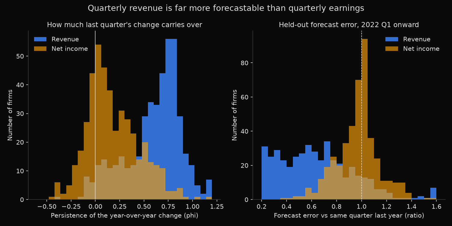
Revenue has memory. Earnings mostly do not. The median φ for revenue is 0.675, so roughly two thirds of a year-over-year revenue gap is still there one quarter later, and 96.4% of firms have a positive coefficient. For net income the median falls to 0.128, and the coefficient is positive at 74.1% of firms, which is far from unanimous.

The gap in raw predictability is wider. Carrying the year-ago quarter forward misses revenue by 10.1% of the firm’s average level and misses net income by 39.5%, roughly four times as much. One operating business, viewed at the top line and at the bottom line, differs fourfold in forecast accuracy.

Adding the Foster term helps only where there was memory to exploit. Median revenue error falls to 0.621 of the naive benchmark, a 38% improvement, and the model beats the benchmark at 87.5% of firms. On net income the median ratio is 0.991 and the win rate is 54.2%, which is close enough to a coin flip that the fitted φ is not carrying information out of sample.

Walmart shows the pattern at its sharpest: revenue missed by 5.1% and net income by 45.1%, from the same quarters of the same company. Sales arrive smoothly, while the bottom line absorbs charges that do not repeat on any schedule. Nvidia sits at the other extreme, with high persistence in both series, 0.967 and 0.816, because a sustained growth run puts a trend into revenue and earnings alike.

So what?

Build the forecast at the top line, then bridge down. Fitting a time-series model to bottom-line dollars means fitting a series whose year-over-year deviations barely persist; a revenue projection plus an explicit margin assumption keeps the predictable part and the judgement part separate.

The naive numbers set the bar. A revenue model that cannot beat 10.1% relative error, or cannot beat the 38% improvement a two-parameter regression delivers, is not paying for its complexity. For earnings, no simple extrapolation clears the bar at all, so the effort belongs in the margin bridge and in the treatment of one-off items.

Store φ per firm rather than applying one number across a portfolio. A company at 0.85 rewards carrying recent growth forward; a company near zero should be forecast at the year-ago level and left there. The estimate has a second use in screening: when a ranking uses trailing earnings as a stand-in for next year’s, 39.5% is the size of the noise that ranking is sorting on.

Built with xfinlink — free financial data API for Python. pip install -U xfinlink