
Does the Balance Sheet Change Which Stocks Look Cheap? P/E Against EV/EBIT in Python
September 12, 2026
What’s the question?
A price-to-earnings ratio prices one claim on a company. It divides the market value of the shares by the profit left after interest and tax, so it describes the equity alone. Enterprise value takes the other view: it adds debt to the share value and subtracts cash, pricing the whole operating business whoever funded it. Set that against operating profit, measured before any interest is paid, and the result is EV/EBIT.
Take two companies earning identical operating profit from identical assets. One funds itself with shareholders’ money and holds cash; the other borrows. Interest charges cut the borrower’s net income and raise its P/E, while the borrowed money sits inside enterprise value and raises its EV/EBIT. Which force wins decides whether the borrower looks cheaper or dearer after the swap.
What matters is how often the disagreement is large enough to change a decision, and whether it lands where capital actually gets committed.
The approach
One cross-section of the S&P 500, valued at the 2025 fiscal year end.
- Take the index membership as it stood on 31 December 2025 and carry every member by entity id, so that a recycled ticker cannot swap one company for another.
- Drop Financials and Real Estate, where debt is raw material rather than funding and an enterprise multiple has no clean meaning.
- Keep companies whose latest annual report covers a fiscal year ending between 1 December 2025 and 31 January 2026, putting every valuation within five weeks of one date.
- Require a reported cash balance, a total debt figure, a diluted share count, positive net income and positive operating profit.
- Require the profit line to reconcile: net income within 10% of pre-tax income minus tax. Minority interests, discontinued operations and preferred dividends break that link, so those names sit outside the comparison.
- Value each company at its own fiscal year end, using that day’s closing price times diluted shares, so price and balance sheet share a date.
That leaves 212 companies, each ranked twice; the gap between the two rank positions is the quantity of interest.
Code
import pandas as pd
from scipy import stats
import xfinlink as xfl

xfl.set_api_key("YOUR_API_KEY")  # free at https://xfinlink.com/signup

AS_OF = "2025-12-31"
FY_LO, FY_HI = "2025-12-01", "2026-01-31"
FIELDS = ["net_income", "ebit", "pretax_income", "income_tax_expense", "total_debt",
          "cash_and_short_term_investments", "weighted_avg_shares_diluted"]

ids = sorted(xfl.index("sp500", as_of=AS_OF)["entity_id"].dropna().astype(int))

a = pd.concat(
    [xfl.fundamentals(entity_id=ids[i:i + 60], period_type="annual",
                      start="2024-06-01", fields=FIELDS, max_rows=200000)
     for i in range(0, len(ids), 60)], ignore_index=True)
a = a.dropna(subset=["period_end"]).drop_duplicates(["entity_id", "period_end"])
f = a.sort_values("period_end").groupby("entity_id").tail(1).set_index("entity_id")
f = f[~f["gics_sector"].isin({"Financials", "Real Estate"})]
f = f[(f["period_end"] >= FY_LO) & (f["period_end"] <= FY_HI)]
f = f.dropna(subset=FIELDS)
f = f[(f["net_income"] > 0) & (f["ebit"] > 0) & (f["weighted_avg_shares_diluted"] > 0)]

gap = (f["net_income"] - (f["pretax_income"] - f["income_tax_expense"])).abs()
f = f[gap <= 0.10 * f["net_income"]]               # profit line must reconcile

px = pd.concat(
    [xfl.prices(entity_id=list(f.index)[i:i + 60], start="2025-12-15", end="2026-02-02",
                fields=["close"], max_rows=200000)
     for i in range(0, len(f), 60)], ignore_index=True)
px = px.dropna(subset=["close"]).sort_values("date")
d = pd.merge_asof(f.reset_index().sort_values("period_end"),
                  px[["entity_id", "date", "close"]], left_on="period_end",
                  right_on="date", by="entity_id",
                  tolerance=pd.Timedelta("7D")).set_index("entity_id")
d = d.dropna(subset=["close"])

d["market_cap"] = d["close"] * d["weighted_avg_shares_diluted"]
d["net_debt"] = d["total_debt"] - d["cash_and_short_term_investments"]
d["ev"] = d["market_cap"] + d["net_debt"]
d = d[d["ev"] > 0]
d["pe"] = d["market_cap"] / d["net_income"]
d["ev_ebit"] = d["ev"] / d["ebit"]
d["nd"] = d["net_debt"] / d["market_cap"]
d["r_pe"] = d["pe"].rank()
d["r_ev"] = d["ev_ebit"].rank()
d["move"] = d["r_pe"] - d["r_ev"]          # positive: cheaper on the enterprise multiple

n, k = len(d), len(d) // 5
q = pd.qcut(d["nd"], 5, labels=False)
cheap = len(set(d.nsmallest(k, "pe").index) & set(d.nsmallest(k, "ev_ebit").index))
dear = len(set(d.nlargest(k, "pe").index) & set(d.nlargest(k, "ev_ebit").index))

print(n, k, d["pe"].median(), d["ev_ebit"].median(), d["nd"].median())
print(stats.spearmanr(d["pe"], d["ev_ebit"]).statistic, cheap, dear, (d["move"].abs() > 50).sum())
print(d.groupby(q).agg(n=("pe", "size"), nd=("nd", "median"), pe=("pe", "median"),
                       ev=("ev_ebit", "median"), move=("move", "median")))
print(d.nlargest(8, "move")[["ticker", "pe", "ev_ebit", "nd", "r_pe", "r_ev"]])
print(d.nsmallest(8, "move")[["ticker", "pe", "ev_ebit", "nd", "r_pe", "r_ev"]])
print(d.groupby("gics_sector").agg(n=("pe", "size"), nd=("nd", "median"),
                                   move=("move", "median")).sort_values("move"))
Full script with formatting and visualisation: pe-versus-ev-ebit-sp500-python.py
Output
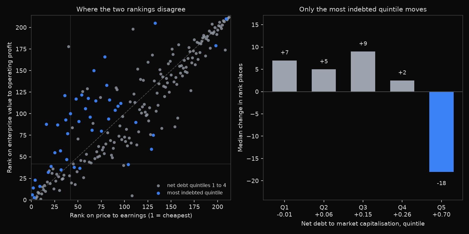
Equity multiple against enterprise multiple, S&P 500 at 31 December 2025
Universe: 497 index members on 2025-12-31, carried by entity id;
          212 non-financial companies with a fiscal year ending
          1 December 2025 to 31 January 2026 and a reconciling profit line
P/E     = diluted market capitalisation / net income
EV/EBIT = (diluted market capitalisation + total debt - cash) / operating profit

Median P/E 25.58      median EV/EBIT 21.26      median net debt / market cap +0.15
Spearman rank correlation between the two multiples   +0.8726

Cheapest quintile (42 names)   32 shared, 10 replaced
Dearest quintile  (42 names)   35 shared, 7 replaced
Companies moving more than 50 rank places: 25 of 212

By net debt quintile (net debt / market capitalisation)
  quintile        net debt   median P/E   median EV/EBIT   median rank move
  1 ( 43 names)     -0.01        32.35            25.48               +7.0
  2 ( 42 names)     +0.06        31.70            25.83               +5.0
  3 ( 42 names)     +0.15        26.92            21.13               +9.0
  4 ( 42 names)     +0.26        21.09            18.51               +2.5
  5 ( 43 names)     +0.70        18.60            20.09              -18.0

Largest moves toward cheap on the enterprise multiple
  ticker  company                          P/E   EV/EBIT   net debt   P/E rank   EV rank
  HUM     HUMANA INC                      26.05     8.66      -0.24        108         5
  SWK     STANLEY BLACK & DECKER INC      28.90    17.82      +0.43        129        59
  BKNG    BOOKING HOLDINGS INC            32.35    19.78      -0.00        154        85
  NCLH    NORWEGIAN CRUISE LINE HLDGS     25.19    15.49      +1.27        104        41
  MAR     MARRIOTT INTERNATIONAL INC      32.63    20.42      -0.00        157        95
  DPZ     DOMINOS PIZZA INC               24.21    15.16      -0.01         99        40
  EPAM    EPAM SYSTEMS INC                30.50    19.71      -0.11        140        83
  SW      SMURFIT WESTROCK PLC            29.10    19.21      +0.62        131        75

Largest moves toward expensive on the enterprise multiple
  ticker  company                          P/E   EV/EBIT   net debt   P/E rank   EV rank
  UBER    UBER TECHNOLOGIES INC           17.23    31.74      +0.02         40       178
  FANG    DIAMONDBACK ENERGY INC          26.12    45.69      +0.33        109       198
  XEL     X C E L ENERGY INC              21.56    29.66      +0.76         79       166
  D       DOMINION ENERGY INC             16.72    22.35      +0.97         36       121
  LNT     ALLIANT ENERGY CORP             20.69    26.58      +0.63         67       150
  GM      General Motors Company          29.34    65.23      +1.40        133       205
  PCG     P G & E CORP                    13.09    19.95      +1.68         16        88
  REGN    REGENERON PHARMACEUTICALS IN    18.61    23.11      -0.01         55       126

By sector
  sector                     names   median net debt   median rank move
  Utilities                    26             +0.75              -35.5
  Communication Services        8             +0.50               -4.0
  Energy                       13             +0.21               -2.0
  Health Care                  30             +0.14               -0.5
  Information Technology       30             +0.03               +0.0
  Materials                    16             +0.19               +6.5
  Consumer Staples             14             +0.20              +12.5
  Industrials                  52             +0.10              +13.0
  Consumer Discretionary       23             -0.01              +16.0
What this tells us
The two rankings agree on the broad shape and disagree at the edges. A Spearman rank correlation of +0.8726 says a company near the cheap end on one measure is usually near the cheap end on the other, yet 25 of the 212 move more than 50 places, and ten of the 42 names in the cheapest quintile on P/E leave it once the balance sheet enters.
The quintile table shows where the disagreement lives. Four of the five net debt buckets barely move, with median rank changes of +7.0, +5.0, +9.0 and +2.5 places against a 212-name list. The most indebted fifth, carrying net debt equal to 0.70 times market value at the median, drops 18 places, and that same bucket holds the lowest median P/E in the sample at 18.60. Borrowing lifts earnings per share and pulls the equity multiple down; the enterprise multiple takes that flattery back out. Utilities carry most of the effect, losing 35.5 rank places on median net debt of 0.75, while Consumer Discretionary gains 16.0 places on net debt near zero.
Two individual cases warn against applying the enterprise multiple mechanically. General Motors moves from 133rd to 205th, but most of its $110bn of net debt funds the loan book at its finance arm rather than its factories, and Humana moves from 108th to 5th on a cash pile that backs insurance claims rather than sitting idle. Uber is cleaner, at 17.23 times earnings against 31.74 times operating profit, because a large tax credit lifted net income above what the business itself earned.
So what?
Screen on P/E for the four-fifths of the market carrying little net debt. An enterprise multiple buys a median of nine rank places or fewer there, which will not change a shortlist.
Inside the most indebted fifth the equity multiple is measuring the funding as much as the business, and a low P/E in that group deserves the enterprise check before anything else. That fifth is mostly regulated utilities and a scattering of heavily borrowed operators, so a value screen filling up with utilities has probably found borrowing rather than value.
Two checks belong with the enterprise multiple. Confirm the cash is genuinely spare rather than regulatory float, and confirm the debt funds operations rather than a captive lending book. Either failure moves EV/EBIT for a reason unrelated to the business being valued.
Built with xfinlink — free financial data API for Python. pip install -U xfinlink
pip install -U xfinlink