Does Covariance Shrinkage Beat the Sample Covariance? Minimum-Variance Portfolios in Python

July 31, 2026

What’s the question?

A minimum-variance portfolio is the set of weights producing the lowest possible variance from a given set of assets. It needs one input: the covariance matrix of returns, never known and always estimated. Thirty assets means 30 variances plus 435 covariances, so one rebalance rests on 465 estimated numbers the optimiser treats as exact.

That is a problem, because minimum-variance weights depend on the inverse of the matrix. Inversion divides by the smallest eigenvalues, exactly the directions where the sample estimate is least reliable. Two stocks that happened to move together during the estimation window look like a free variance reduction, so the optimiser takes a large long position in one and a large short in the other. When the correlation reverts, that pair stops cancelling and starts contributing risk.

Ledoit and Wolf proposed the standard repair in 2004: mix the sample matrix with a structured target, here a scaled identity matrix that assumes equal variances and zero correlation everywhere. The target is wrong, but it carries no estimation error, and a weighted average of a noisy unbiased estimate and a clean biased one can beat both. The mixing weight, called the shrinkage intensity, comes from the data.

The approach

The universe is the current 30 members of the Dow Jones Industrial Average, pulled from the index endpoint. Every name is live and trades on every day of the sample, giving a complete panel of 1,255 trading days across calendar years 2021 through 2025.

1. Every 21 trading days, estimate the covariance matrix from a trailing window of daily returns.
2. Build four portfolios: equal weight, minimum variance on the sample matrix, minimum variance on the shrunk matrix, and minimum variance on the sample matrix with weights held non-negative.
3. Hold each for the following 21 trading days. No information from the holding period enters the weights.
4. Repeat with estimation windows of 252 and 60 days, keeping the out-of-sample period fixed at 987 days so the runs are comparable.

Estimating 465 parameters from 252 observations is already thin; at 60 observations there are two data points per asset. If shrinkage is worth anything, the short window is where it should show.

Code

import numpy as np
import pandas as pd
from scipy.optimize import minimize
import xfinlink as xfl

xfl.set_api_key("YOUR_API_KEY")  # free at https://xfinlink.com/signup

tickers = sorted(xfl.index("djia")["ticker"].tolist())
px = xfl.prices(tickers, start="2021-01-01", end="2025-12-31", fields=["return_daily"])
R = px.pivot(index="date", columns="ticker", values="return_daily").sort_index().dropna()
X, N = R.to_numpy(), R.shape[1]


def ledoit_wolf(Z):
    """Shrink the sample covariance toward a scaled identity matrix."""
    T, n = Z.shape
    Zc = Z - Z.mean(axis=0)
    S = Zc.T @ Zc / T
    mu = np.trace(S) / n
    d2 = np.sum((S - mu * np.eye(n)) ** 2) / n
    b2 = (np.sum(np.einsum("ij,ij->i", Zc, Zc) ** 2) - T * np.sum(S ** 2)) / (n * T ** 2)
    a = float(np.clip(b2 / d2, 0.0, 1.0))
    return a * mu * np.eye(n) + (1 - a) * S, a


def min_var(cov):
    w = np.linalg.solve(cov, np.ones(len(cov)))
    return w / w.sum()


def min_var_long_only(cov):
    n = len(cov)
    return minimize(lambda w: w @ cov @ w, np.repeat(1 / n, n),
                    jac=lambda w: 2 * cov @ w, method="SLSQP",
                    bounds=[(0.0, 1.0)] * n,
                    constraints=[{"type": "eq", "fun": lambda w: w.sum() - 1.0}]).x


for window in (252, 60):
    oos = {k: [] for k in ("equal", "sample", "shrunk", "long_only")}
    for t in range(252, len(X) - 20, 21):
        train, test = X[t - window:t], X[t:t + 21]
        S = np.cov(train, rowvar=False)
        LW, intensity = ledoit_wolf(train)
        oos["equal"].append(test @ np.repeat(1 / N, N))
        oos["sample"].append(test @ min_var(S))
        oos["shrunk"].append(test @ min_var(LW))
        oos["long_only"].append(test @ min_var_long_only(S))

    for k, v in oos.items():
        r = np.concatenate(v)
        print(window, k, "vol %.2f%%" % (r.std(ddof=1) * np.sqrt(252) * 100))

Full script with formatting and visualisation: covariance-shrinkage-minimum-variance-portfolio-python.py

Output

=== SANITY ===
tickers: 30 | trading days: 1255
range: 2021-01-04 -> 2025-12-31 | monotonic: True
NaNs in matrix: 0
min daily return: -0.2238  max daily return: 0.2437
obs with |return| > 20%: 3
    2024-07-26 MMM 0.2299
    2023-05-25 NVDA 0.2437
    2025-04-17 UNH -0.2238

=== 252-DAY ESTIMATION WINDOW: 47 rebalances, 987 out-of-sample days, 30 assets ===
Portfolio                   Vol   Return   Sharpe    Gross   MaxWgt  Shorts
Equal weight             15.58%   12.56%     0.81     1.00     3.3%     0.0
Min-var, sample cov      13.06%    4.73%     0.36     1.75    21.3%     9.9
Min-var, shrunk cov      12.75%    5.24%     0.41     1.55    17.3%     8.8
Min-var, long-only       12.36%    6.31%     0.51     1.00    19.8%     0.0
Mean shrinkage intensity: 0.078   Vol change, shrunk vs sample: -2.4%

=== 60-DAY ESTIMATION WINDOW: 47 rebalances, 987 out-of-sample days, 30 assets ===
Portfolio                   Vol   Return   Sharpe    Gross   MaxWgt  Shorts
Equal weight             15.58%   12.56%     0.81     1.00     3.3%     0.0
Min-var, sample cov      17.01%    7.20%     0.42     3.11    36.2%    11.8
Min-var, shrunk cov      12.87%    5.94%     0.46     1.59    15.6%     7.8
Min-var, long-only       12.75%    7.51%     0.59     1.00    26.2%     0.0
Mean shrinkage intensity: 0.251   Vol change, shrunk vs sample: -24.3%

=== CHECKS ===
window 252 | max |sum(w)-1| = 4.4e-16 | min long-only weight = 0.0e+00 | shrinkage 0.024-0.138 | max cond(S) = 215 | NaNs = 0
window  60 | max |sum(w)-1| = 4.4e-16 | min long-only weight = 0.0e+00 | shrinkage 0.068-0.518 | max cond(S) = 1377 | NaNs = 0

What this tells us

The value of shrinkage depends almost entirely on how much data the covariance estimate is built from.

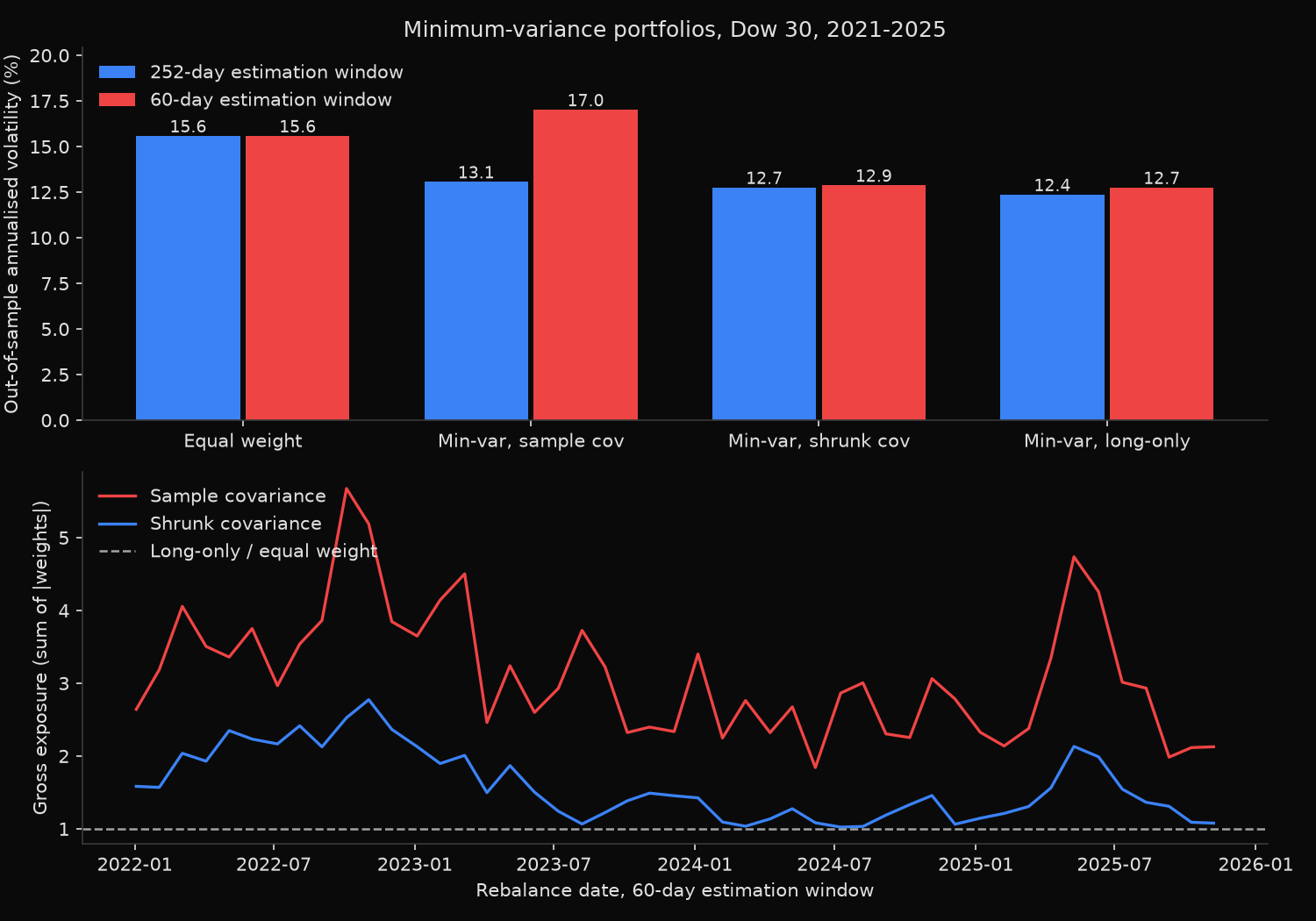
On the 252-day window the sample matrix is already good enough. Minimum variance on it delivered 13.06% realised volatility against 15.58% for equal weight, and shrinkage improved that to 12.75%. Average intensity was 0.078, so the estimator gave the sample matrix 92% of the weight; with a condition number peaking at 215, that judgement is right, and shrinkage earns about 30 basis points.

The 60-day window inverts the result. Minimum variance on the sample matrix produced 17.01% realised volatility, worse than naive equal weighting: a procedure whose purpose is to minimise variance ended up increasing it. The lower panel shows why. Gross exposure averaged 3.11 with peaks above 5.5, the average largest position was 36.2%, and the optimiser financed its phantom hedges with 11.8 short positions, working from a matrix whose condition number reached 1,377. Shrinkage cut volatility to 12.87%, a 24.3% reduction, and pulled gross exposure to 1.59 as average intensity rose to 0.251.

The long-only portfolio is the quiet winner. It never touched the shrinkage code, yet delivered 12.36% and 12.75% volatility at the two windows. Jagannathan and Ma showed in 2003 that a non-negativity constraint is mathematically equivalent to shrinking the covariance matrix, since each binding constraint acts like a reduction in the estimated covariances of the asset it excludes. Forbidding shorts stabilised the portfolio as effectively as the explicit estimator.

One number cuts against all three optimised portfolios: equal weight produced the highest Sharpe ratio in every run, 0.81 against a range of 0.36 to 0.59, because it held the high-volatility, high-return names minimum variance avoids by construction.

So what?

Check the ratio of observations to assets before choosing an estimator. At roughly eight observations per asset the sample covariance matrix works and shrinkage is a small refinement worth ten lines of code. At two observations per asset it is actively harmful, and the resulting portfolio can carry more risk than one built on no estimate at all.

Anyone wanting minimum-variance exposure without maintaining an estimator has a simpler route: impose a long-only constraint. It delivered the lowest realised volatility of any portfolio tested here, at both window lengths, with gross exposure fixed at 1.00. Gross exposure of 3.11 is not a modelling artefact; it is a borrow and financing bill that no volatility number above includes.

The lesson generalises past minimum variance. Any optimiser inverting an estimated matrix, mean-variance and risk parity included, inherits the same amplification of estimation error. Constrain the output, shrink the input, or estimate fewer parameters; doing none of the three produces a portfolio optimal only in the sample it was fitted to.