
Does Mean-Variance Optimisation Beat Equal Weighting? Out-of-Sample Test in Python
September 8, 2026
What’s the question?
Mean-variance optimisation asks for two inputs: a vector of expected returns and a covariance matrix describing how the holdings move together. Hand it both and it returns the weights with the highest expected return per unit of risk. Markowitz published the method in 1952 and it still underpins institutional asset allocation.
Neither input can be observed. Both are estimated from past returns, and the optimiser cannot tell estimation error from signal, so a stock that happened to post a high average return over the window is read as a stock with a high expected return and bought as heavily as the constraints allow. DeMiguel, Garlappi and Uppal put the consequence sharply in 2009: of the fourteen optimised models they evaluated across seven datasets, none was consistently better than the naive 1/N rule.
Two questions follow. Does an optimised portfolio beat holding the same stocks in equal weight once it is scored on data it never saw, and if it earns anything, which of the two inputs earns it? The second admits a controlled experiment: a minimum-variance portfolio uses the covariance matrix alone, a maximum-Sharpe portfolio uses the covariance matrix and the estimated means, so running both under identical constraints on identical stocks prices the mean vector directly. Sharpe ratios below are annualised mean return over annualised standard deviation, zero risk-free rate throughout.
The approach
- On 1 January of each year from 2006 to 2024, take the S&P 500 as it stood on that date, from a point-in-time membership record, carrying each company by entity id so that a ticker reassigned later cannot substitute one company for another. Draw 150 members at random.
- Estimate the mean vector and the sample covariance matrix from 60 monthly total returns ending the previous December. Names without a complete 60-month series leave the sample, leaving 133 to 147 companies per year.
- From that pool draw 10, 25, 50 or 100 stocks and build three books on them: equal weight, minimum variance, maximum Sharpe. All are long only with weights summing to one, so no shorting and no borrowing.
- Hold for twelve months, resetting to target weights each month. A holding that stops trading part-way through the year hands its weight to the survivors from that month on.
- Repeat with 20 independent draws at each size, then chain the nineteen holding years into a 228-month record per draw.
The long-only constraint is not a detail. Unconstrained weights fitted to 60 months run to enormous offsetting long and short positions that almost no mandate permits, and the restriction acts as a form of shrinkage in its own right; Jagannathan and Ma showed in 2003 that a no-short-sale constraint lowers the realised risk of an estimated optimal portfolio even when the constraint itself is wrong.
Code
import numpy as np
import pandas as pd
import xfinlink as xfl
from scipy.optimize import minimize

xfl.set_api_key("YOUR_API_KEY")  # free at https://xfinlink.com/signup

YEARS, SIZES, DRAWS = range(2006, 2025), [10, 25, 50, 100], 20


def min_variance(S):                        # covariance matrix only
    n = len(S)
    r = minimize(lambda w: w @ S @ w, np.ones(n) / n, jac=lambda w: 2 * S @ w,
                 bounds=[(0.0, 1.0)] * n, method="SLSQP",
                 constraints=[{"type": "eq", "fun": lambda w: w.sum() - 1.0,
                               "jac": lambda w: np.ones(n)}],
                 options={"maxiter": 400, "ftol": 1e-12})
    w = np.clip(r.x, 0, None)
    return w / w.sum()


def max_sharpe(mu, S):                      # covariance matrix and expected returns
    n = len(mu)                             # min y'Sy s.t. mu'y = 1, y >= 0, then rescale
    y0 = np.maximum(mu, 0.0)
    y0 = y0 / (y0 @ mu) if y0 @ mu > 0 else np.ones(n) / n
    r = minimize(lambda y: y @ S @ y, y0, jac=lambda y: 2 * S @ y,
                 bounds=[(0.0, None)] * n, method="SLSQP",
                 constraints=[{"type": "eq", "fun": lambda y: y @ mu - 1.0,
                               "jac": lambda y: mu}],
                 options={"maxiter": 400, "ftol": 1e-12})
    y = np.clip(r.x, 0, None)
    return y / y.sum()


rows = []
for y in YEARS:
    roster = xfl.index("sp500", as_of=f"{y}-01-01")
    ids = sorted({int(x) for x in roster["entity_id"].dropna()})
    pick = sorted(np.random.default_rng(y).choice(ids, 150, replace=False).tolist())
    px = pd.concat([xfl.prices(entity_id=pick[i:i + 50], start=f"{y - 5}-01-01",
                               end=f"{y}-12-31", interval="1mo",
                               fields=["return_daily"], max_rows=200000)
                    for i in range(0, len(pick), 50)], ignore_index=True)
    px["m"] = pd.to_datetime(px["date"]).dt.to_period("M")
    R = (px.drop_duplicates(["entity_id", "m"])
           .pivot(index="m", columns="entity_id", values="return_daily").sort_index())
    est, oos = R[R.index.year <= y - 1], R[R.index.year == y]
    pool = [c for c in R.columns if est[c].notna().all()]
    E, O = est[pool].values, oos[pool].values
    for n in SIZES:
        for k in range(DRAWS):
            sel = np.random.default_rng(y * 1000 + n * 10 + k).choice(len(pool), n, False)
            Xe, Xo = E[:, sel], O[:, sel]
            mu, S = Xe.mean(0), np.cov(Xe, rowvar=False)
            books = {"1/N": np.ones(n) / n, "Minimum variance": min_variance(S),
                     "Maximum Sharpe": max_sharpe(mu, S)}
            live = ~np.isnan(Xo)
            for name, w in books.items():
                held = (live * w).sum(axis=1)   # a name that stops trading hands its weight on
                rows.append({"n": n, "draw": k, "book": name,
                             "in_sample": (w @ mu) / np.sqrt(w @ S @ w) * np.sqrt(12),
                             "rets": np.nansum(np.where(live, Xo, 0.0) * w, 1) / held})

df = pd.DataFrame(rows)
for n in SIZES:
    for name in ["1/N", "Minimum variance", "Maximum Sharpe"]:
        g = df[(df["n"] == n) & (df["book"] == name)]
        r = np.mean(np.stack([np.concatenate(gg["rets"].values)
                              for _, gg in g.groupby("draw")]), axis=0)
        print(f"{n:4d}  {name:18s} in-sample SR {g['in_sample'].mean():5.2f}   "
              f"out-of-sample SR {r.mean() / r.std(ddof=1) * np.sqrt(12):5.3f}")
Full script with formatting and visualisation: mean-variance-vs-equal-weight-out-of-sample-python.py
Output
====================================================================================
WHAT MEAN-VARIANCE OPTIMISATION PROMISES AND WHAT IT DELIVERS
====================================================================================
Universe   S&P 500 point-in-time roster on 1 January of each year, 2006-2024,
           carried by entity id; 150 members drawn per year, of which those with a
           complete 60-month return history form the pool
Estimation 60 monthly total returns ending the December before each rebalance
Holding    the next 12 months, weights held at target, 20 random draws per size
Sharpe     annualised, zero risk-free rate, on the pooled 228-month series

Pool of complete-history names per year: min 133, median 141, max 147
Optimiser convergence: 100.0%   portfolio months with no priced holding: 0

Portfolios of 10 stocks, 60 months of history
                       return      vol   Sharpe      draw range  promised SR  eff names   top wt
  1/N                  9.74%   18.29%    0.603    0.31 to 0.73         0.86       10.0    10.0%
  Minimum variance     9.69%   13.76%    0.744    0.26 to 1.03         1.08        3.9    40.2%
  Maximum Sharpe      10.56%   15.47%    0.730    0.19 to 0.78         1.49        3.2    46.5%

Portfolios of 25 stocks, 60 months of history
                       return      vol   Sharpe      draw range  promised SR  eff names   top wt
  1/N                  9.82%   17.82%    0.617    0.45 to 0.75         0.91       25.0     4.0%
  Minimum variance     9.01%   13.26%    0.720    0.51 to 0.82         1.34        5.9    30.1%
  Maximum Sharpe       9.82%   14.83%    0.709    0.46 to 0.72         1.92        4.8    34.5%

Portfolios of 50 stocks, 60 months of history
                       return      vol   Sharpe      draw range  promised SR  eff names   top wt
  1/N                 10.05%   18.01%    0.624    0.55 to 0.67         0.93       50.0     2.0%
  Minimum variance     9.92%   12.95%    0.799    0.52 to 0.88         1.55        7.5    24.6%
  Maximum Sharpe      10.41%   14.46%    0.760    0.53 to 0.90         2.24        6.1    28.7%

Portfolios of 100 stocks, 60 months of history
                       return      vol   Sharpe      draw range  promised SR  eff names   top wt
  1/N                  9.86%   18.06%    0.614    0.56 to 0.64         0.95      100.0     1.0%
  Minimum variance     9.26%   13.42%    0.730    0.62 to 0.85         1.78        9.2    21.4%
  Maximum Sharpe       9.50%   15.00%    0.682    0.48 to 0.78         2.67        7.4    24.7%

Sharpe against the same stocks held in equal weight, draw by draw
    stocks          minimum variance            maximum Sharpe     means add
        10    +0.074 (13/20 draws)       +0.027 (12/20 draws)        -0.047
        25    +0.050 (14/20 draws)       +0.018 (13/20 draws)        -0.031
        50    +0.124 (19/20 draws)       +0.070 (16/20 draws)        -0.054
       100    +0.094 (19/20 draws)       +0.042 (16/20 draws)        -0.052
  ('means add' is maximum Sharpe minus minimum variance: the payoff to estimating
   expected returns rather than using the covariance matrix alone)
====================================================================================
What this tells us
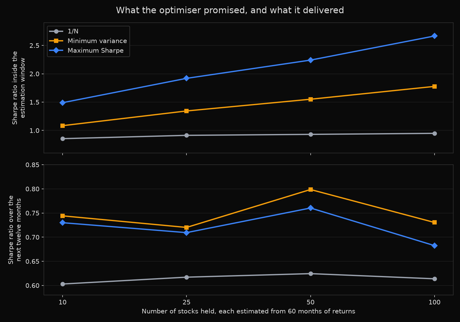
Constrained optimisation cleared the equal-weight benchmark at every size tested. At 50 holdings minimum variance scored a Sharpe of 0.799 and maximum Sharpe 0.760, against 0.624 for the same fifty stocks held equally. The advantage came from one place: annualised volatility fell from 18.01 percent to 12.95 percent while the return barely moved, 9.92 percent against 10.05 percent. The optimiser did not find better stocks. It found a quieter way to hold the ones it was given.
The gap between promise and delivery widens with the size of the problem. A ten-stock maximum-Sharpe book showed a Sharpe of 1.49 inside its estimation window and delivered 0.73; a hundred-stock book showed 2.67 and delivered 0.68. Each added stock is another free parameter, so the fitted figure climbs while the delivered figure does not move.
Now the controlled comparison. Estimating expected returns lifted the promised Sharpe from 1.55 to 2.24 at 50 holdings and from 1.78 to 2.67 at 100, and delivered nothing. Maximum Sharpe finished below minimum variance at all four sizes, and paired draw by draw, so that both books hold exactly the same stocks, it lost by 0.047, 0.031, 0.054 and 0.052. The covariance matrix survived the crossing into live data; the mean vector, fitted from the same 60 months, did not.
Two numbers qualify the result. The minimum-variance edge over equal weight peaks at 50 holdings, worth 0.124 Sharpe points and positive in 19 of 20 draws, and falls to 0.094 at 100, where sixty observations cannot support a covariance matrix for a hundred assets. And that 50-stock book carries an average top weight of 24.6 percent and an effective count of 7.5 names, one over the sum of squared weights.
So what?
Drop the expected return vector. Minimum variance beat maximum Sharpe at all four sizes, on the pooled series and draw for draw alike, while needing half the inputs, and it does so for a structural reason: a covariance matrix is fitted from thousands of pairwise products, a mean from sixty numbers per stock. Research spent forecasting expected returns for an optimiser is spent on the input that failed.
Judge an optimiser by its delivered Sharpe, never its fitted one. A promised 2.67 on 100 assets and 60 observations is arithmetic on an over-fitted problem, and the honest reading of it is 0.68.
Keep the asset count well under the observation count; the ratio governs this, not the count. A hundred-name book rebalanced on five years of monthly data wants a longer window, weekly returns, or a covariance matrix shrunk toward a structured target.
Size the concentration before committing capital. The volatility reduction repeats across draws, but it arrives with a quarter of the book in one name. A mandate capping single-name weight at 5 percent is running a different portfolio from the one tested above, and it deserves its own test.
Built with xfinlink — free financial data API for Python. pip install -U xfinlink
pip install -U xfinlink