Do High Dividend Yields Come From Bigger Payouts or Falling Prices? Yield Decomposition in Python

July 27, 2026

What's the question?

Dividend yield is dividends per share divided by share price. Both halves move, and they carry opposite messages. A stock yielding 5% because management has raised the payout for a decade is a different proposition from one yielding 5% because the price fell by half. A yield screen cannot tell them apart, because it only sees the ratio.

The arithmetic is exact. Taking logs of yield = DPS / price and differencing across two dates gives:

log(y_2025 / y_2020) = log(DPS_2025 / DPS_2020) - log(P_2025 / P_2020)

A change in yield is dividend growth minus price return, with no residual. The empirical question follows: across the S&P 500, which term decides where a company sits in today’s yield ranking?

The approach

The sample is S&P 500 constituents with a December fiscal year end, which puts every company on the same two dates, 31 December 2020 and 31 December 2025.

1. Pull annual dividend_yield for both fiscal years, keeping the rows that end on those exact dates.
2. Pull adj_close for both dates. It is split-adjusted and gap-free, so a split cannot masquerade as a price move.
3. Merge on entity_id rather than ticker, so a symbol changing hands cannot splice two companies into one.
4. Keep names yielding at least 1% at both ends. Below that a dividend is a rounding error.
5. Require the annual dividend per share to reconcile with the company’s own quarterly record, within 25%, at both anchors. Some filers carry the quarterly column year to date, so the rebuild differences the running total first.
6. Require the symbol to have belonged to the same company at the 2020 anchor, and that anchor quote to be confirmable for it.
7. Compute the price leg as the negative log price ratio, then take the payout leg as the remainder.
8. Sort by 2025 yield into quintiles and compare the median of each leg.

Steps 5 and 6 are ordinary hygiene: an anchor that is wrong for one company distorts every statistic that company enters, and a five-year window offers two chances to go wrong.

Of 499 constituents, 347 have a December year end with data at both dates and 189 clear the yield floor. Three then fail the reconciliation and one the anchor check, leaving 185, of which 183 carry a full quarterly record to test against. Finally, yield multiplied by the year-end close should reproduce each company’s reported dividend per share, and it does for all 185, within 2%.

Code

import numpy as np
import pandas as pd
from scipy.stats import spearmanr
import xfinlink as xfl

xfl.set_api_key("YOUR_API_KEY")  # free at https://xfinlink.com/signup

START, END = "2020-12-31", "2025-12-31"
RECON_TOL = 0.25
universe = sorted(xfl.index("sp500")["ticker"].dropna().unique().tolist())


def chunked(fetch, tickers, size=50):
    return pd.concat([fetch(tickers[i:i + size])
                      for i in range(0, len(tickers), size)], ignore_index=True)


def annual_yield(date):
    m = chunked(lambda b: xfl.metrics(b, period_type="annual", start=date[:4] + "-01-01",
                                      end=date, fields=["dividend_yield"]), universe)
    return m[m["period_end"] == date].drop_duplicates("entity_id")


def close_on(date):
    start = (pd.Timestamp(date) - pd.Timedelta(days=16)).date().isoformat()
    p = chunked(lambda b: xfl.prices(b, start=start, end=date,
                                     fields=["close", "adj_close"]), universe)
    return p.sort_values("date").drop_duplicates("entity_id", keep="last")


def dividends_from_quarters(year, tickers):
    """Rebuild a fiscal year's dividend per share from the quarterly record."""
    q = chunked(lambda b: xfl.fundamentals(b, period_type="quarterly", start=f"{year}-01-01",
                                           end=f"{year}-12-31",
                                           fields=["dividends_per_share"]), tickers)
    q = q.dropna(subset=["dividends_per_share"]).drop_duplicates(
        ["entity_id", "fiscal_year", "fiscal_period"])
    w = (q.pivot_table(index="entity_id", columns="fiscal_period",
                       values="dividends_per_share")
          .reindex(columns=["Q1", "Q2", "Q3", "Q4"]).dropna())
    # some filers carry the quarterly column year to date rather than standalone;
    # differencing the running total recovers the same annual figure either way
    running = (w["Q2"] > w["Q1"] * 1.6) & (w["Q3"] > w["Q2"] * 1.4)
    return pd.Series(np.where(running, 2 * w["Q3"] - w["Q2"], w.sum(axis=1)),
                     index=w.index, name="rebuilt")


y_end, y_start = annual_yield(END), annual_yield(START)
p_end, p_start = close_on(END), close_on(START)

# entity_id, not ticker: a symbol can change hands between the two dates
d = (y_end[["entity_id", "dividend_yield"]].rename(columns={"dividend_yield": "y1"})
     .merge(y_start[["entity_id", "dividend_yield"]].rename(columns={"dividend_yield": "y0"}),
            on="entity_id")
     .merge(p_end[["entity_id", "ticker", "gics_sector", "close", "adj_close"]].rename(
         columns={"close": "c1", "adj_close": "a1"}), on="entity_id")
     .merge(p_start[["entity_id", "close", "adj_close"]].rename(
         columns={"close": "c0", "adj_close": "a0"}), on="entity_id"))

d = d[(d["y0"] >= 0.01) & (d["y1"] >= 0.01)].copy()

for year, y, c in [(2020, "y0", "c0"), (2025, "y1", "c1")]:
    d = d.join(dividends_from_quarters(year, sorted(d["ticker"].tolist())), on="entity_id")
    gap = (d[y] * d[c] / d["rebuilt"] - 1).abs()
    d = d[(gap <= RECON_TOL) | d["rebuilt"].isna()].drop(columns="rebuilt")

d["price_leg"] = -np.log(d["a1"] / d["a0"])
d["yield_leg"] = np.log(d["y1"] / d["y0"])
d["payout_leg"] = d["yield_leg"] - d["price_leg"]

cov = np.cov(np.vstack([d["yield_leg"], d["payout_leg"], d["price_leg"]]))
print("price leg share of variance:", round(cov[0, 2] / cov[0, 0], 3))
print("rank corr, 2025 yield vs price change:", round(spearmanr(d["y1"], -d["price_leg"])[0], 3))

d["quintile"] = pd.qcut(d["y1"], 5, labels=[1, 2, 3, 4, 5])
pct = lambda s: np.expm1(s.median()) * 100
print(d.groupby("quintile", observed=True).agg(
    n=("entity_id", "size"),
    yield_2025=("y1", lambda s: s.median() * 100),
    dps_growth=("payout_leg", pct),
    price_change=("price_leg", lambda s: np.expm1(-s.median()) * 100)))

Full script with the anchor check, formatting and visualisation: dividend-yield-payout-price-decomposition-python.py

Output

S&P 500 constituents: 499
December fiscal year end with both snapshots: 347
Yielding at least 1% at both ends: 189
Dropped, annual and quarterly dividend records disagree: 3
Dividend record reconciled for 183 of the 186 remaining; the rest carry no full quarterly record to test against
Dropped, anchor date not confirmable for the same company: 1
Final sample: 185
Dividend-per-share cross-check: 185 names, 100.0% agree within 2%

S&P 500 dividend payers, five-year yield decomposition (medians)
quintile  n   yield 2020  yield 2025  DPS growth  price change
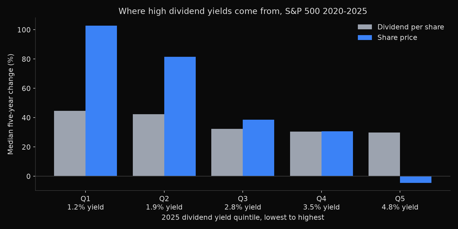
    1     37        1.7%        1.2%       44.7%       102.8%
    2     37        2.4%        1.9%       42.3%        81.5%
    3     37        3.0%        2.8%       32.4%        38.6%
    4     37        3.6%        3.5%       30.4%        30.6%
    5     37        4.1%        4.8%       29.8%        -4.5%

Price leg carries 76.6% of the cross-sectional variance in yield changes
Payout leg carries 23.4%
Spearman rank correlation, 2025 yield vs five-year price change:  -0.499
Spearman rank correlation, 2025 yield vs five-year DPS growth:    -0.197

Sector, share of its dividend payers landing in the top yield quintile
  Communication Services    3 of  4      75%
  Real Estate              14 of 24      58%
  Consumer Staples          3 of 11      27%
  Health Care               2 of  9      22%
  Energy                    4 of 18      22%
  Utilities                 4 of 23      17%
  Consumer Discretionary    1 of  7      14%
  Materials                 2 of 16      12%
  Financials                3 of 41       7%
  Industrials               1 of 27       4%
  Information Technology    0 of  5       0%

What this tells us

The payout column barely moves. Median dividends per share rose 44.7% in the lowest-yield quintile and 29.8% in the highest, a spread of 15 points. Every quintile raised its dividend, the top one by close to a third. Nothing there looks like distress.

The price column is a different picture. The lowest-yield quintile more than doubled, at +102.8%, while the highest finished five years below where it started, at -4.5%. That spread is 107 points, seven times the payout spread, and it falls monotonically down the table.

The variance decomposition puts a number on it: 76.6% of the cross-sectional variation in five-year yield changes traces to the price leg, 23.4% to the payout leg. Rank correlations agree, at -0.499 for the 2025 yield against five-year price change and only -0.197 against dividend growth.

The sector table shows part of the mechanism. 14 of the 24 real estate names sit in the top yield quintile, against 1 of 27 industrials and none of the 5 technology names. Communication Services reads 3 of 4, too thin a base to read anything into. Sorting on yield is a sector bet arrived at indirectly.

So what?

A high-yield screen is largely a price screen wearing a payout label. That is not an argument against owning high yielders, but an argument for knowing what the position is: such a screen overweights names the market has de-rated and underweights names that compounded. Whether that is value or a value trap is the analyst’s call, and it should be a deliberate choice rather than a side effect of the sort.

Two things follow. Decompose before screening and rank on the leg the mandate cares about; the identity above separates a dividend raised through a flat tape from a tape that simply fell. Then check the sector exposure of a yield-sorted portfolio before sizing it, because the sort concentrates in real estate and drains industrials and technology.

Yield reports what the market thinks of a company at least as much as what the company pays. Reading it as the second alone discards most of the information in it.