
What’s the question?
Share repurchases are the largest single use of corporate cash in the American equity market, and the case for them rests on one number that nobody reports. A buyback converts cash into a smaller share count. Whether that helps the remaining holders depends entirely on the price paid: buying below what the business is worth transfers value from the sellers to the holders, and buying above it runs the transfer the other way. The dollars spent are disclosed every year. The price those dollars bought at is not. How those programmes are financed, from free cash flow or from new borrowing, is the question in a buyback funding analysis.
Management is the party with the best information about the business, which suggests a testable prediction. If that information advantage extends to the company’s own valuation, repurchase spending should rise when the stock is cheap and fall when it is expensive.
Measuring this requires separating the timing of spending from its size. A company that repurchases 10 billion dollars over a decade is neither better nor worse at timing than one that repurchases 100 million, and the raw average price paid says more about which decade the company existed in than about any decision it made. The comparison that isolates timing is against the company’s own alternative: spending the identical amount every year. That benchmark requires no forecast and no skill, so any gap between the two is attributable to when the money went out. A company that does spend evenly scores exactly 1.000 by construction, which makes the score readable without reference to anything else.
The approach
The sample is the S&P 500 as it stood on 31 December 2015, addressed by entity identifier rather than ticker so that a later rename or delisting does not drop the company from the sample. Fiscal years 2015 through 2024 give ten annual observations of repurchase spending from the cash flow statement.
- Keep companies reporting positive repurchases in at least five of the ten fiscal years. A programme active in fewer years than that has too few observations for a timing measurement to mean anything.
- Take monthly split-adjusted closes and average them within each company’s own fiscal year. An adjusted price is the price per current-equivalent share, so dollars divided by an adjusted price gives shares on today’s terms, and a split partway through the sample does not distort the arithmetic.
- Compute the dollar-weighted average price as total dollars divided by total shares acquired, where shares acquired in a year is that year’s spending divided by that year’s average price.
- Compute the equal-dollar average price the same way, holding spending constant across the same fiscal years. The ratio of the two is the score.
The score has one property worth stating plainly before the numbers arrive: it depends only on the relationship between spending and price, never on the price path itself. A company whose stock quadrupled and a company whose stock halved both score 1.000 if their spending was flat.
Code
import numpy as np
import pandas as pd
import xfinlink as xfl

xfl.set_api_key("YOUR_API_KEY")  # free at https://xfinlink.com/signup

roster = xfl.index("sp500", as_of="2015-12-31")
ids = sorted(set(int(i) for i in roster["entity_id"].dropna()))

fun = xfl.fundamentals(entity_id=ids, start="2014-06-30", end="2025-12-31",
                       period_type="annual", fields=["share_repurchases"],
                       max_rows=40000)
fun["period_end"] = pd.to_datetime(fun["period_end"])
fun = fun[(fun["fiscal_year"] >= 2015) & (fun["fiscal_year"] <= 2024)]
fun = fun[fun["share_repurchases"] > 0]
counts = fun.groupby("entity_id").size()
keep = counts[counts >= 5].index.tolist()

px = xfl.prices(entity_id=keep, start="2014-01-01", end="2025-12-31",
                interval="1mo", fields=["adj_close"], max_rows=200000)
px["date"] = pd.to_datetime(px["date"])

rows = []
for eid, g in fun[fun["entity_id"].isin(keep)].groupby("entity_id"):
    p = px[px["entity_id"] == eid]
    recs = []
    for _, r in g.iterrows():
        end = r["period_end"]
        w = p[(p["date"] > end - pd.Timedelta(days=364)) & (p["date"] <= end)]
        if len(w) >= 10:
            recs.append((float(r["share_repurchases"]), float(w["adj_close"].mean())))
    if len(recs) < 5:
        continue
    d = np.array([x[0] for x in recs])
    pr = np.array([x[1] for x in recs])
    dollar_weighted = d.sum() / (d / pr).sum()
    equal_dollar = len(pr) / (1.0 / pr).sum()
    rows.append({"ticker": g["ticker"].iloc[-1], "dollars": d.sum(),
                 "score": dollar_weighted / equal_dollar})

res = pd.DataFrame(rows)
print(res["score"].median(), (res["score"] > 1).mean())
Full script with formatting and visualisation: buyback-timing-dollar-weighted-price-python.py
Output
S&P 500 members at 2015-12-31, fiscal years 2015-2024
companies with >=5 repurchase years and usable prices: 377
company-years 3256   total repurchased $6.34 trillion

timing score (1.000 = spent evenly; above 1 = paid more than even spending would)
  median            1.0535
  mean              1.1356
  share above 1.0   74.5%
  dollar-weighted   1.1253
  quartiles         0.999 / 1.053 / 1.146

by sector
                         n  median  dollars
sector
Energy                  23  1.2016    290.0
Materials               21  1.0741    100.0
Consumer Discretionary  55  1.0708    604.0
Communication Services  12  1.0702    574.0
Information Technology  45  1.0673   1608.0
Health Care             46  1.0592    690.0
Financials              62  1.0497   1420.0
Real Estate             15  1.0420     26.0
Industrials             58  1.0419    633.0
Utilities                8  1.0279     11.0
Consumer Staples        32  1.0204    383.0

the twelve largest programmes
ticker                   name  years  dollars    score
  AAPL              Apple Inc     10    657.7 1.277538
 GOOGL           ALPHABET INC     10    302.2 1.619037
  MSFT         MICROSOFT CORP     10    195.0 1.186155
  META     Meta Platforms Inc      8    147.7 1.180073
  ORCL            ORACLE CORP     10    128.5 0.967020
   WFC       WELLS FARGO & CO     10    127.1 1.074493
   JPM    JPMORGAN CHASE & CO      9    125.2 1.044103
   BAC   BANK OF AMERICA CORP     10    123.4 1.142735
     V               VISA INC     10     90.0 1.180735
     C          CITIGROUP INC     10     79.5 1.074689
   BRK BERKSHIRE HATHAWAY INC      7     77.9 0.960922
  CSCO      CISCO SYSTEMS INC     10     73.5 1.067279

best and worst timers among programmes above $5bn
  best   MSI 0.742, YUM 0.837, GLW 0.839, MCD 0.861, PH 0.864, ABBV 0.881
  worst  NVDA 3.792, GE 1.741, KLAC 1.693, CCL 1.638, ADBE 1.625, GOOGL 1.619

aggregate spending against the sample's median share price
             dollars  price_index
fiscal_year
2015           455.0        100.0
2016           530.0        101.9
2017           480.0        111.6
2018           711.0        120.7
2019           696.0        129.9
2020           457.0        134.1
2021           706.0        162.7
2022           843.0        168.4
2023           708.0        159.2
2024           754.0        180.1
What this tells us
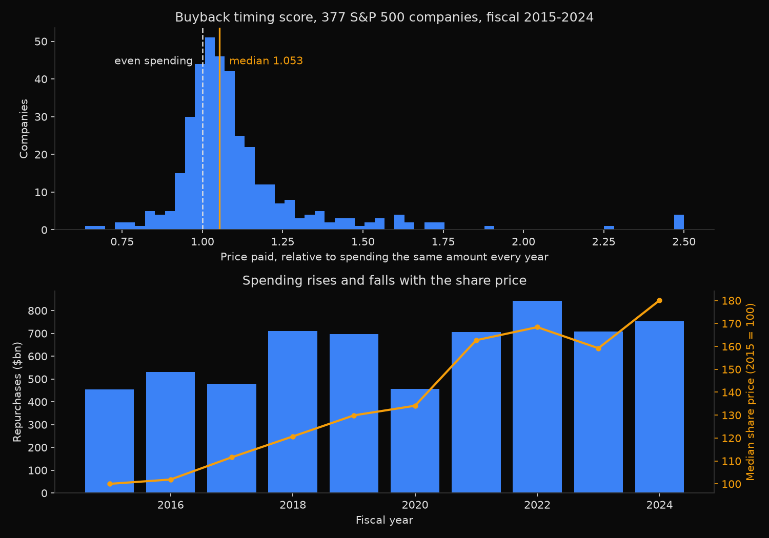
The prediction fails, and it fails in the same direction almost everywhere. Three quarters of the 377 companies score above 1.000, the median company paid 5.4 percent more than flat spending would have, and weighting by dollars raises the penalty to 12.5 percent because the largest programmes are among the worst timed. Across 6.34 trillion dollars of repurchases, the timing decision destroyed value rather than adding it.
The bottom panel of the chart shows the mechanism directly. Spending ran at 455 billion dollars in fiscal 2015 with the sample’s median share price at 100, and at 754 billion in fiscal 2024 with that price at 180. The two series move together, and the one year where spending collapsed, fiscal 2020, was the year prices were closest to a trough. Repurchases are funded out of current cash flow, and cash flow is strongest exactly when business conditions and share prices are both good, so the spending pattern follows the balance sheet rather than the valuation.
Every sector scores above 1.000, which rules out an explanation resting on any single industry. Energy is worst at 1.202, consistent with a sector that generated enormous free cash flow in 2022 and 2023 and spent it while prices were high. Consumer staples is closest to even at 1.020, which is what steady cash flow through a cycle produces without anyone deciding anything.
The individual programmes carry the sharpest version. NVIDIA scores 3.792: it repurchased across seven fiscal years and concentrated the money in the two most expensive of them. Alphabet at 1.619 and Apple at 1.278 spent hundreds of billions on the same pattern. Two names run the other way, and both are the ones an observer would guess: Berkshire Hathaway at 0.961 and Oracle at 0.967. Berkshire’s programme is explicitly conditioned on price, and it is one of the few here where the score suggests the condition binds.
So what?
Treat a buyback announcement as a statement about cash on hand, not as a signal that management considers the shares cheap. The evidence says the two coincide only by accident, and the accident runs the wrong way about three quarters of the time.
For anyone valuing a company, the score is worth computing before assuming a repurchase programme accretes value. It needs one line of the cash flow statement and a price series, and a decade of history gives enough observations to separate a genuine policy from a coincidence. A company scoring below 1.000 over ten years has demonstrated something the large majority of the index has not.
For anyone holding shares, the practical consequence is in the payout mix. Repurchases at 12.5 percent above an even-spending benchmark are a materially worse way to return capital than dividends of the same size, which carry no timing decision at all. That is the case against buybacks stated in numbers rather than in principle, and it applies to the aggregate rather than to any particular company: a quarter of these programmes did beat the benchmark.
Built with xfinlink — free financial data API for Python.