Does the Piotroski F-Score Still Work? Quality Screening in Python

August 20, 2026

What’s the question?

The Piotroski F-Score is nine yes-or-no accounting tests applied to a company’s last two annual reports. Four ask about profitability: is net income positive, is operating cash flow positive, did return on assets improve, does cash flow exceed net income. Three ask about the balance sheet: did leverage fall, did the current ratio improve, did the share count avoid growing. Two ask about operations: did gross margin improve, did asset turnover improve. Each pass scores a point, giving a total from 0 to 9.

Joseph Piotroski introduced it in 2000 as a way to sort cheap stocks, and the original result was strong: among high book-to-market companies, the ones with clean accounting signals substantially outperformed the ones without. Twenty-six years later the score is in every screening tool, which is exactly the condition under which a published anomaly stops paying. The question here is whether the score still separates next year’s winners from its losers inside the S&P 500, where the companies are large, widely covered, and rarely distressed.

The approach

Eight annual formation dates, one twelve-month holding period each, measured on price returns.

1. Take the S&P 500 roster as it stood on 30 June for each year from 2018 to 2025, so companies later removed from the index stay in the sample
2. Attach each company’s F-Score from the most recent fiscal year that ended at least six months before the formation date, which keeps the test to figures that had already been reported
3. Drop financials, real estate and utilities, since the leverage and asset-turnover tests are built for non-financial balance sheets
4. Sort the remainder into three buckets: low (0-3), middle (4-6) and high (7-9)
5. Measure the twelve-month price return from 30 June to the following 30 June and compare bucket medians and hit rates

That gives 2,825 company-years. The low bucket is thin by construction, at 159 company-years, because index membership itself screens out most companies with deteriorating accounts.

Code

import pandas as pd
import xfinlink as xfl

xfl.set_api_key("YOUR_API_KEY")  # free at https://xfinlink.com/signup

rosters = {y: xfl.index("sp500", as_of=f"{y}-06-30") for y in range(2018, 2026)}
universe = sorted({t for r in rosters.values() for t in r["ticker"].dropna()})

sframes, pframes = [], []
for i in range(0, len(universe), 100):
    batch = universe[i:i + 100]
    sframes.append(xfl.metrics(batch, period_type="annual", start="2016-01-01",
                               end="2026-08-19", fields=["piotroski_f_score"],
                               max_rows=300000))
    pframes.append(xfl.prices(batch, start="2017-12-01", end="2026-08-19",
                              interval="1mo", fields=["adj_close"], max_rows=500000))

scores = pd.concat(sframes).dropna(subset=["piotroski_f_score"])
scores["period_end"] = pd.to_datetime(scores["period_end"])

px = pd.concat(pframes)
px["month"] = pd.to_datetime(px["date"]).dt.to_period("M")
last = px.sort_values("date").groupby(["entity_id", "month"], as_index=False).last()
panel = last.pivot(index="month", columns="entity_id", values="adj_close")
sector = last.groupby("entity_id")["gics_sector"].last()

rows = []
for year in range(2018, 2026):
    known = scores[scores["period_end"] <= pd.Timestamp(f"{year}-01-01")]
    latest = known.sort_values("period_end").groupby("entity_id").last()
    ids = [i for i in rosters[year]["entity_id"]
           if i in panel.columns and i in latest.index
           and sector.get(i) not in {"Financials", "Real Estate", "Utilities"}]
    m0, m1 = pd.Period(f"{year}-06", "M"), pd.Period(f"{year + 1}-06", "M")
    ret = (panel.loc[m1, ids] / panel.loc[m0, ids] - 1).dropna()
    rows.append(pd.DataFrame({"f": latest.loc[ret.index, "piotroski_f_score"],
                              "ret": ret, "year": year}))

pool = pd.concat(rows)
pool["bucket"] = pd.cut(pool["f"], [-0.1, 3, 6, 9],
                        labels=["low 0-3", "middle 4-6", "high 7-9"])
print(pool.groupby("bucket", observed=True)["ret"].agg(
    ["size", "median", "mean", lambda s: (s > 0).mean()]))

Full script with formatting and visualisation: piotroski-f-score-forward-returns-python.py

Output

Pooled 12-month price returns, 2825 company-years, 8 formation dates
            names  median_pct  mean_pct  positive_pct
bucket
low 0-3       159         5.3      12.0          53.5
middle 4-6   1616         5.7      12.3          56.4
high 7-9     1050         7.9      13.7          61.7

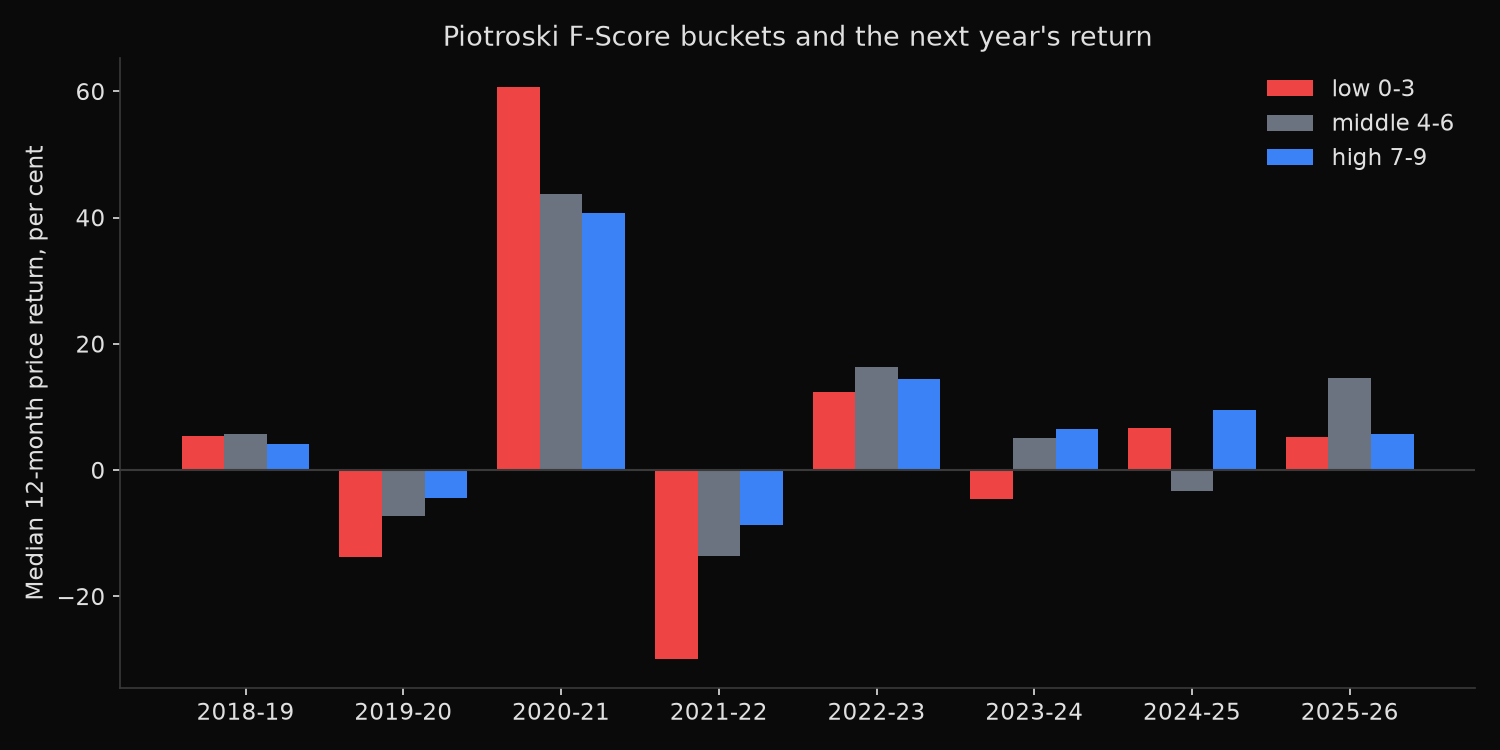
Median 12-month price return by formation year, per cent
bucket  low 0-3  middle 4-6  high 7-9  high - low
year
2018        5.3         5.7       4.1        -1.2
2019      -13.7        -7.3      -4.5         9.2
2020       60.7        43.8      40.8       -19.9
2021      -29.9       -13.6      -8.7        21.3
2022       12.4        16.3      14.4         2.1
2023       -4.6         5.1       6.6        11.2
2024        6.7        -3.3       9.5         2.8
2025        5.3        14.6       5.7         0.5

High minus low spread positive in 6 of 8 years, median 2.4 points

What this tells us

Pooled across all eight years the ordering holds, and it is smaller than the score’s reputation suggests. Median returns rise from 5.3% to 7.9% moving from the low bucket to the high one, a gradient of 2.6 percentage points over a full year. Means rise from 12.0% to 13.7%. Both orderings are monotone, and neither is large enough to build a strategy on by itself.

The hit rate is the more informative column. High-scoring companies finished the year up 61.7% of the time against 53.5% for low-scoring ones, a gap of 8.2 points, which is three times the gradient in median return. The score is telling you more about the probability of a bad year than about the size of a good one. That is what an accounting-quality signal should do, and it matches the mechanics: none of the nine tests measures growth, valuation or momentum, so none of them predicts a large upside move.

Year by year the spread is unreliable. It favoured high scores in six of the eight years with a median of 2.4 points, and the two exceptions are the ones that matter. In the year from June 2020 the low bucket returned a median 60.7% against 40.8% for the high bucket, a 19.9-point inversion, because a recovery rally off a crash pays most to the companies whose accounts looked worst at the bottom. The following year reversed it exactly, with the low bucket down 29.9% against 8.7% for the high bucket. The signal is a bet against distress, and that bet loses precisely when distress is being rewarded.

So what?

Treat the F-Score as a risk filter rather than a return engine. Excluding the bottom bucket removes companies carrying a 46.5% chance of a down year and keeps ones carrying 38.3%, which is a meaningful improvement in the shape of a portfolio’s outcomes and a negligible one in its expected return. Screening on it and expecting alpha will disappoint.

The regime dependence is the part to size around. Any strategy that ranks on accounting quality is short distress risk, so it will underperform in the first year of a recovery and outperform in a drawdown. Pairing it with a signal that behaves the opposite way, such as a valuation or reversal measure, is a better use than running it alone.

Inside a large-cap index the score also has less to work with than Piotroski’s original setting gave it. His result came from high book-to-market companies, where accounting deterioration is common and cheaply priced. The S&P 500 selects those companies out before the screen ever sees them, which compresses the dispersion the score depends on. On a small-cap or a deep-value universe the same test deserves a fresh measurement rather than an assumption that this result carries over.

Built with xfinlink — free financial data API for Python. pip install -U xfinlink